Column Charts

Introduction:

Excel is not just used for organizing and processing data and formulas. It also can be used to visually represent data in the form of charts and graphs. Column charts are useful for showing data changes over a period of time or for illustrating comparisons among items. In column charts, categories are typically organized along the horizontal axis and values along the vertical axis, as long as the data are limited to approximately twenty categories or less.

Learning:

A clustered column chart is sometimes called a bar graph, because it shows data organized in solid shapes like pillars, with each rectangular bar with lengths proportional to the values that they represent. A clustered column chart organizes these pillars up and down, so they are “columns.” On the other hand, a clustered bar graph organizes these pillars horizontally, so they are “bars.” Each bar graph will plot categories versus frequency of occurrences within the category.

The first step to creating any chart is to organize your data. It is definitely a good idea to include headers in the first cell of each column. By default, a column chart will cluster the data by the columns in your table, so try to keep that in mind when setting up the worksheet.

After organizing your data, select the cells you wish to include in the chart. This should be at least two columns.

Click on the Insert tab and find the Charts group of the ribbon. You

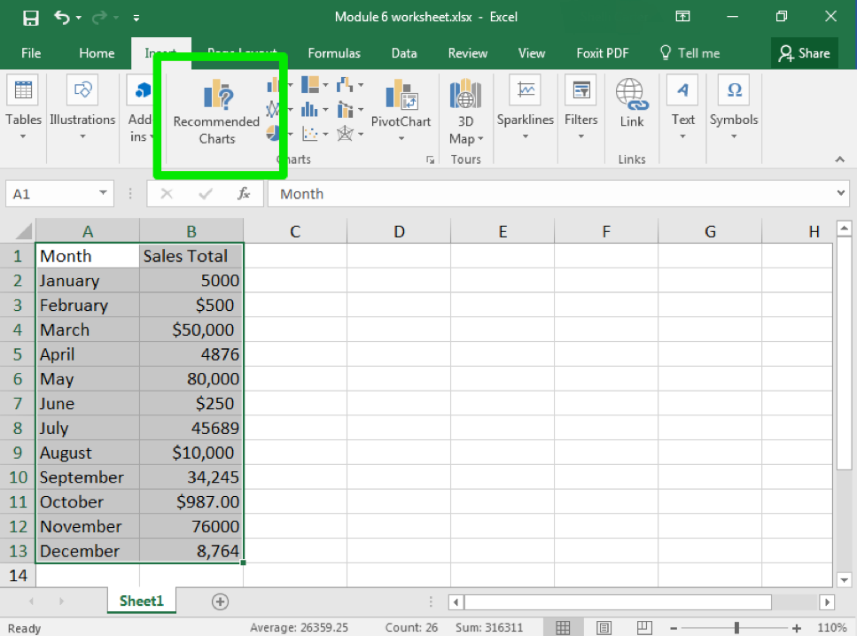
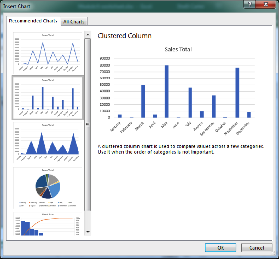
“Clustered column chart” is actually a recommended chart. Click on that chart.

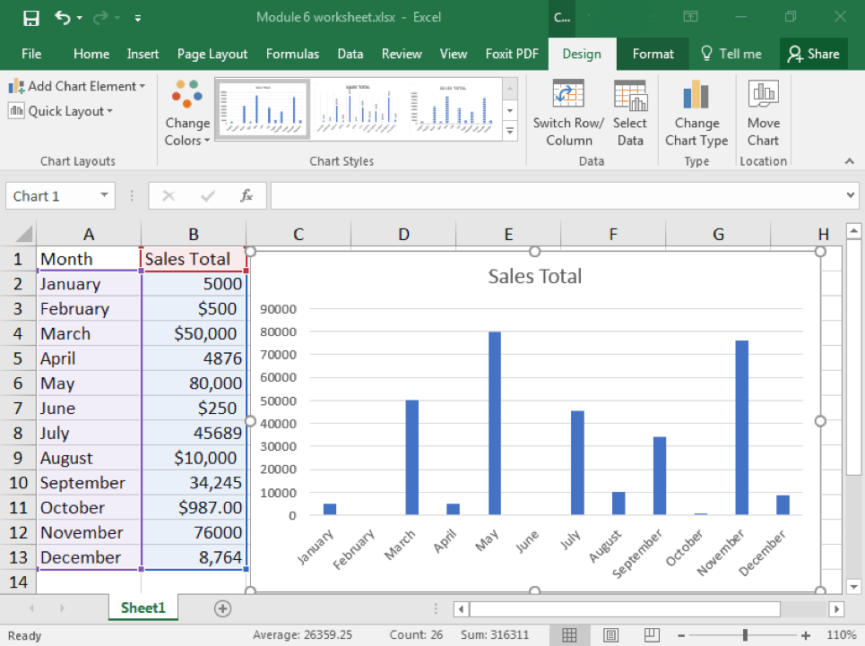
When you select the chart, you will see colored boxes surrounding the data that connect to the different categories of the chart.

The recommended chart option is clearly a time saver, but knowing some of the options is important as well. Let’s explore the Insert Chart options for Column charts. Note that Bar charts have similar options to the Column charts, but will be horizontal instead of vertical.

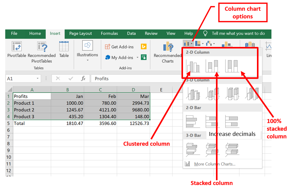
For the above example, by default each row represents the categories that will appear on the X axis. The Columns of data represent the series on the chart: Column B (Jan) is series1, Column C (Feb) is series2, and Column D (Mar) is series 3.

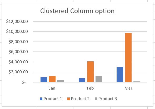
The first option of the column charts is called a Clustered column. For a clustered column, each series is shown side by side for each category. This chart is preferred when trying to show the relative differences of series within the category.

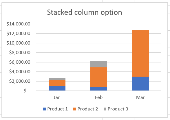
The second option is called a stacked column. For the stacked column, each series is stacked on top of each other for each category. The advantage of using this type of chart, is that the height of the stacked bars also indicates the Total amount of the category. Use this chart when you have multiple data series and you want to emphasize the total.

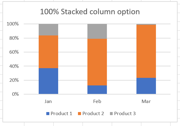
The third option is called 100% stacked column. Even though it isn’t used often, the chart does have relevance when you have two or more data series and you want to emphasize the contributions to the whole, especially if the total is the same for each category. Each height of the stacked bars is the same, and the relative size of each series within the category are shown as percentage of 100%.

Use the Chart Tools Design tab and Chart Tools Format tab (which are Contextual tabs – only show up when a chart is selected) to adjust Titles, axis labels, and other formatting options for the charts.

Summary:

Column and Bar charts are some of the most often produced charts in Excel. The Column chart shows data in vertical bars, and the Bar chart shows data in horizontal bars. The process to insert column (or bar) charts is to select the data that is intended to be graphed, click on the Insert Tab, and use either the Recommended chart or select the desired chart from the Charts group.

Sources:

Clustered Charts. Authored by: Shelli Carter. Provided by: Lumen Learning. License: CC BY 4.0