Tables

Introduction:

Data in cells that are in a range (located adjacent to each other) can be converted to a table for ease of filtering and sorting. There are several advantages to converting your range to a table which include preset formats and filtering and sorting options. To make sure your data can be converted to a table make sure there are no blank rows or columns.

Learning:

One very common task in Excel is to format a table with a particular style. The controls for table styles are found in the Styles group of the ribbon under the Home tab.

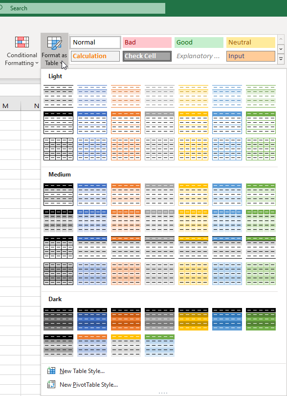
There are many default table styles within Excel, as shown in the screenshot below. Among other uses, styles let you apply color schemes to tables that can make them more readable. In order to apply a particular table style:

• Select all the cells that belong in your table.
• Click on the “Format as Table” button.
• Choose which table style to apply.

When applying the table style, be sure to check the box if your table has headers that you have already entered.

Converting Data Ranges to Tables

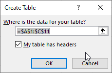
To convert a data range to a table, select any cell in your data range and click the Format as Table button in the Styles group of the Home tab on the Ribbon. From the drop-down menu select the desired table view from the options and then select if your table has headers from the Format as Table dialog box and click ok to create a table from your data range.

You can also create a table from data by using the Table button found in the Tables group on the Insert tab of the Ribbon.

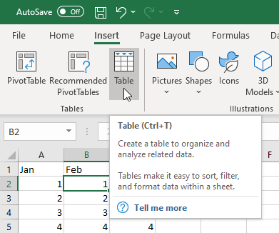
The difference between the two options is the first allows the user to select different coloring options instead of the default table colors used by the Table button on the Insert tab.

You will need to tell Excel if your table has headers or not before completing the conversion to a table.

If you wish to add data to a table simply begin adding data below the last row of the table and Excel will incorporate it into the table, applies the correct formatting and formulas to the newly entered data.

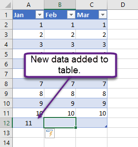
Note: If your data range contains blank rows or columns Excel may not correctly choose which information to include in the table.

Filtering and Sorting Data in Tables

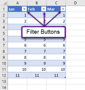
Each column header now has a Filter button (drop-down arrow) which allows you to filter and sort the data quickly using the menu provided.

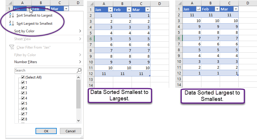
Sorting a table adjusts the rows by the selection in the Filter button in that column. This can be done by clicking the Filter button in a column header and using the Sort Smallest to Largest / Sort Largest to Smallest or Sort AZ / ZA options in the menu (these options vary depending on the data contained in the column). The sorting of data in a single column rearranges all the rows in the table. When the data in a column has been sorted the Filter, button displays a different icon, noting that this column has been sorted.

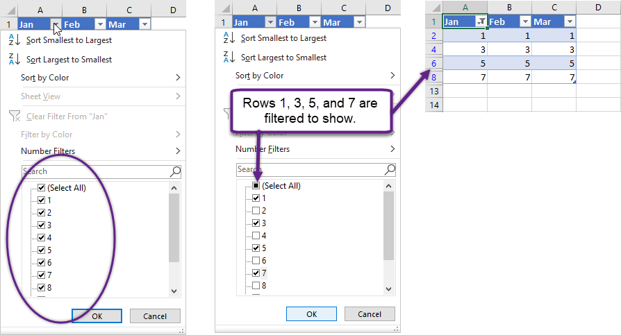
Filtering a table adjusts the rows by only showing the rows that meet the criteria chosen for filtering. Rows that do not meet the filter criteria are hidden (these rows are NOT deleted from the table.) The process is to select the Filter button in a column header and using the Filter options that are at the bottom of the menu. To hide rows and filter them out of the data set, uncheck the box associated with the data you do not wish to show. If there is a large amount of data, you can click the Select All check box to deselect all the options and check off the ones you want to show up on the table. Just like sorting a table filtering a table also changes the Filter button icon to identify that this column has been filtered.

Multiple filtering and sorting can be done on tables to provide the data you are seeking. To clear sorting and filtering you click on the Filter button in the header and select Clear Filter from the menu options. For multiple filters and sorts you can clear all of them by using the Sort & Filter button in the Editing group of the Home tab of the Ribbon. In the Sort & Filter menu choose Clear to clear multiple filters and sorts at one time.

Converting Tables to Data Ranges

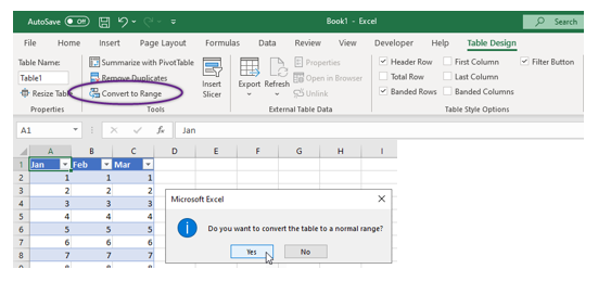
Sometimes you create a table and do not want to keep working with the table functionality that it comes with. Instead, you want something that looks like a table (i.e. formatting). To keep data in a table without losing formatting, convert the table to a regular range of data. To do this, select anywhere in the table you wish to convert to a range, this will generate the Table Design contextual menu on the Ribbon. From that contextual tab, in the Tools group, click Convert to Range and your table will return to a data range but keep the colored formatting of the table.

Summary:

Converting data ranges to tables provides an easy way to filter and sort data if the data range meets the right criteria. Sorting adjusts rows to display data in a specific way whereas filtering hides unwanted data from the table display. Each of these options can be used together or separately.

Sources:

IDM