Lab Week 3 – Overhead Cost Analysis

Background

Now that you have determined you are able to join Longmeadow Baking Company if you can pay yourself $1000 per week, and have determined the starting inventory costs, it is time to determine the business overhead costs* you expect to incur. *The review of overhead costs is not a comprehensive examination, but a quick glimpse at some of the factors associated with overhead found in a business.

Goal

For this assignment, you are going to put together a list of overhead expenses using round numbers to approximate what you may spend if you join Longmeadow Baking Company. This information will also help us determine how much we should charge for our baked goods in future analysis.

After you complete your Overhead Costs Analysis, you wanted to get a graphical representation of the expenses you estimated to use in your decision to join Longmeadow Baking Company. To accomplish this, we are going to insert two different charts (a pie chart and a bar chart) that calculate the expenses without the calculation of the salary.

You will demonstrate the following Excel skills with this exercise:

• Applying formatting (column width, row height, fill, font, alignment, number, styles)
• Format painter
• Basic formula creation
• Copy/paste formula
• Basic functions (SUM, AVERAGE, MIN, MAX)
• Chart creation (Clustered column, Pie Chart)
• Worksheet management

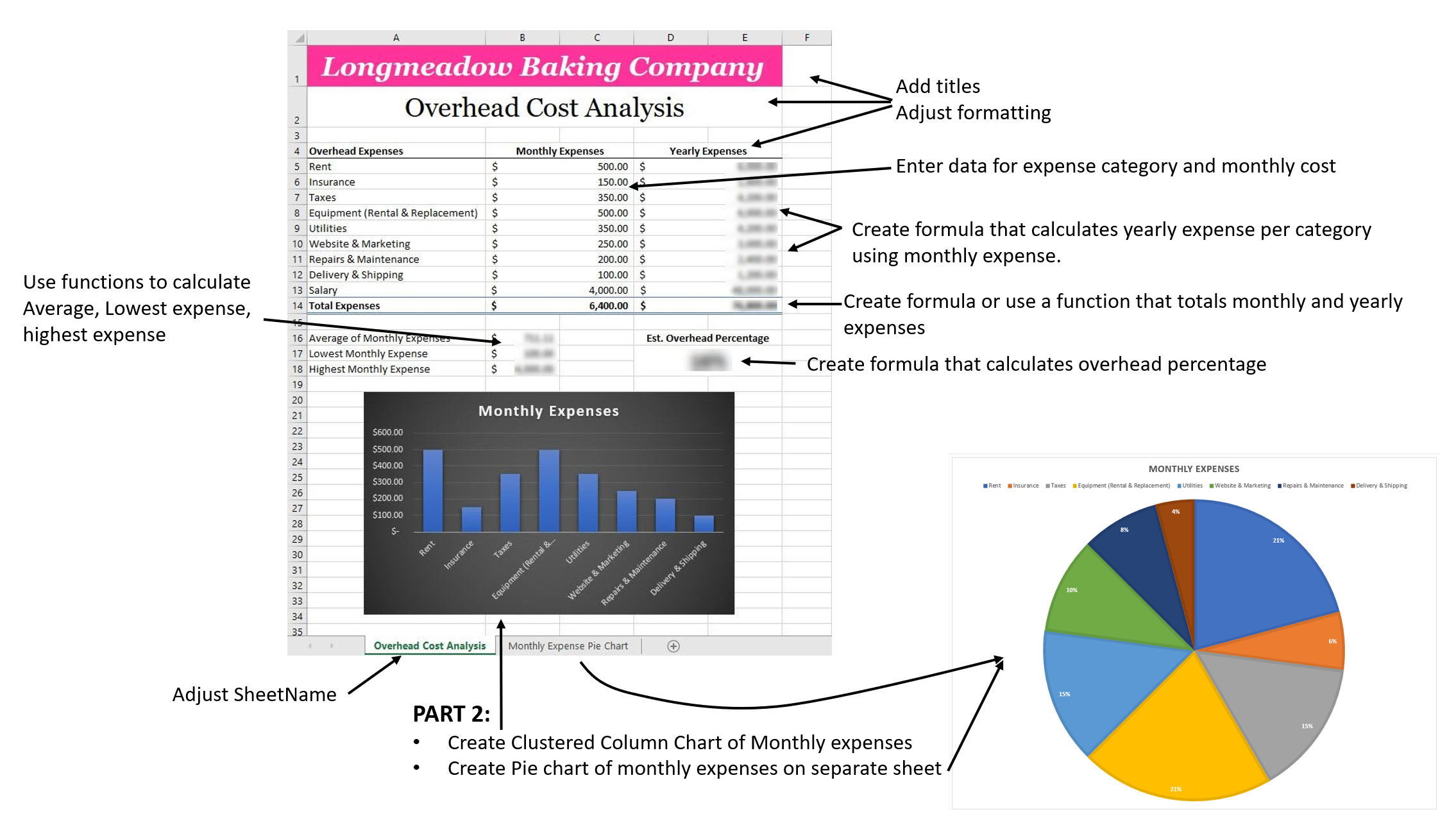
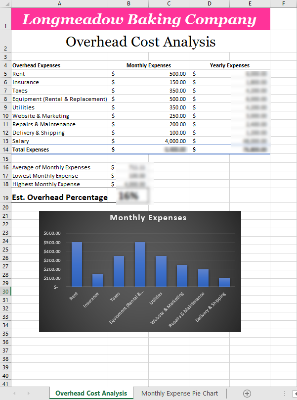
The completed spreadsheet should look like this:

Calculating Overhead Percentage

1. Open Microsoft Excel and create a new workbook and name it “Overhead Cost Workbook.xlsx”

2. Enter the following text in:
   1. cell A1: Longmeadow Baking Company
   2. cell B2: Overhead Cost Analysis
   3. cell A4: Overhead Expenses
   4. cell B4: Monthly Expenses
   5. cell D4: Yearly Expenses
3. Enter the following data into your worksheet beginning in cell A5:B13:

4. Save your workbook.

5. Auto-Adjust the width of column A
6. Columns B:E width = 13
7. Rows 1 & 2 height = 40
8. Merge and Center cells A1:E1
9. Formatting adjustments for cell A1:
   1. Georgia Pro 26, Bold, White, and Italic
   2. fill color #FF3399 (more color options menu)
   3. Middle-align alignment (title centered within the cell)
10. Merge and Center cells A2:E2
11. Formatting adjustments for cell A2:
    1. Georgia Pro 26, Bold
    2. Middle-align alignment (title centered within the cell)
12. Merge and Center cells B4:C4 and cells D4:E4
13. Change the font in cells in row 4 (cells A4, B4:C4 and D4:E4) to Bold and add a bottom border
14. Merge and Center cells B5:C5 to B14:C14 and change the number format to Accounting
15. Merge and Center the cells D5:E5 to D14:E14 and change the number format to Accounting

16. Create a formula in D5 to calculate the Yearly Expenses (Monthly Expenses X 12). Copy and paste the Formula from cell D5 to cells D6:D13, making sure to maintain formatting when you copy and paste.
17. In Row 14, use a Function to calculate the total of the Monthly Expenses and Yearly Expenses

18. Bold the data in cells A14:E14
19. Apply the Total Cell Style from the Styles Group on the Home Tab to cells A14:E14

20. In cell A16 enter the following text: Average of Monthly Expenses. In cell B16 use the AVERAGE Function to calculate the average (include salary in the calculation)
21. In cell A17 enter the following text: Lowest Monthly Expenses. In cell B17 use the MIN Function to calculate the lowest expense
22. In cell A18 enter the following text: Highest Monthly Expenses. In cell B18 use the MAX Function to calculate the highest expense
23. Format the results in cells B16:B18 to Accounting format

Based on the information that your potential partners at Longmeadow Baking Company have provided, you can estimate sales of roughly $10,000 per week ($40,000 per month). Although actual sales may vary, we are going to use this number to determine the percentage of overhead we should include in our product pricing to maintain our margins. The calculation for determining overhead as a percentage is the Total Monthly Expenses / Estimated Monthly Sales.

24. Enter the text: Ext. Overhead Percentage in cell A19. Make the text bold and 16 point.
25. In cell B19, create a formula to calculate overhead percentage:

*note: adjust format to % and Bold, 20 pt, middle-aligned

26. Rename the worksheet tab to Overhead Cost Analysis
27. Save your workbook.

Adding Charts to Visualize the Data

1. Continue using your “Overhead Cost Workbook.xlsx” file.
2. Save your workbook.

3. Highlight your expenses (minus the salary) in columns A and B:C
4. Insert a Clustered Column Chart using the Recommended Charts option
5. With the Clustered Column Chart selected, move it underneath your table and center it with the top of the chart at the top of row 21
6. Change the Chart Title to Monthly Expenses
7. Change the Chart Style to “Style 8”

8. Highlight your all the expenses (minus the salary) in columns A and B:C
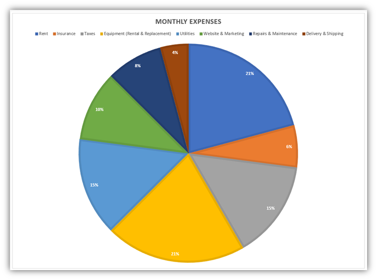
9. Insert a Pie Chart using the Recommended Charts option
10. Change the Chart Title to Monthly Expenses
11. Change the Chart Style to “Style 8”
12. Move the Pie Chart to a New Sheet and change the worksheet label to Monthly Expense Pie Chart
13. Move the Monthly Expense Pie Chart worksheet to the Right of the Overhead Cost Analysis worksheet
14. Save your workbook as and close Excel