Lab Week 4 – Food Cost Analysis
Background
After concluding last week our estimated sales, overhead costs, and our estimated overhead percentage, we now need to price out how much it will cost us to produce our cakes, cupcakes, and cookies. This information will be vital in understanding how much we are going to spend in creating each of our recipes and further help with the decision to join the Longmeadow Baking Company.
Goal
In this assignment, you are going to evaluate a list of vendors and ingredients to get the best price for your cakes, cupcakes, and cookies. You will enter this information into a table to determine the price per ounce and unit.
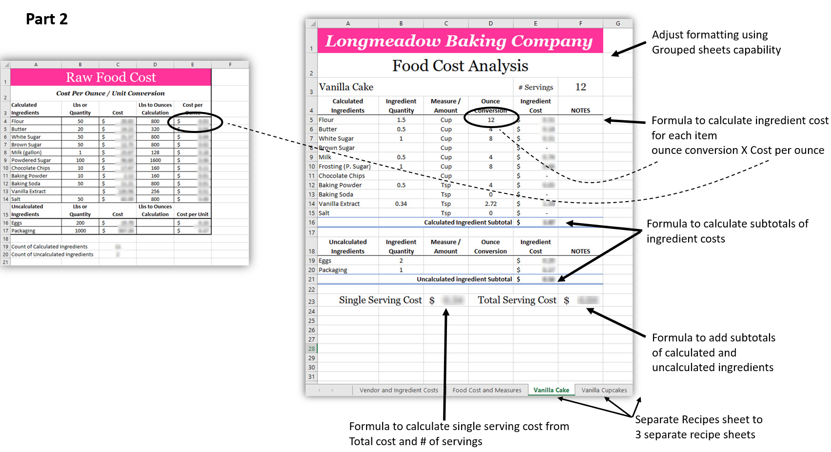
Then you will enter the ingredient prices into your three recipes (provided) and calculate how much it costs to create each baked good and the cost of an individual serving. This information will be used to determine how much you should charge for your baked goods.
You will demonstrate the following Excel skills with this exercise:
- Applying formatting (column width, row height, fill, font, alignment, number, styles)
- Format painter
- Basic formula creation
- Copy/paste formula
- Basic functions (COUNT)
- Excel Tables
- Filtering
- Relative and Absolute cell referencing
- Worksheet management
- Renaming worksheets
- Grouping worksheets
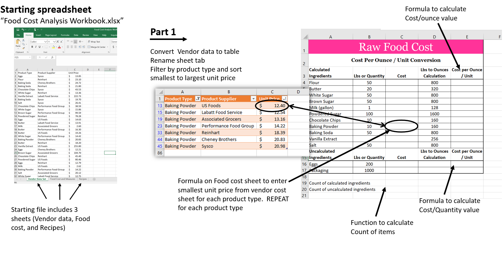
You’ll be completing this spreadsheet over the next two weeks. You’ll work on Part 1 this week, and Part 2 next week. The completed spreadsheet will eventually be:
Evaluating vendors and pricing
- Download (from your Canvas module) and open the starting workbook “Food Cost Analysis Workbook.xlsx”
- Save the workbook as
first initial.last name Food Cost Analysis Part 1
(example: W. Jones – Food Cost Analysis Part 1).
- On the Vendor Data Set worksheet, select all the data in columns A:C
- Convert the selected data into a Table, using Orange, Table Style Medium 3, with Headers included (Styles Group on the Home Tab)
- Rename the Vendor Data Set worksheet to “Vendor and Ingredient Costs”
- You need to find the minimum price for each product type. One way to do this is to Filter the data by Product Type (one product type at a time) and then filter the data by Unit Price, smallest to largest (see example below: be sure to filter by Product Type first, then filter the data by Unit Price).
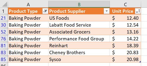
For this case, the minimum Unit Price for “Baking Powder” is in cell C21.
Let’s Check Your Process…
- On the Food Cost & Measures worksheet:
- Create a Relative Cell Reference to the corresponding ingredient’s minimum unit Cost cell (Column C).
- Let’s create the first one together for the Calculated Ingredient, Flour.
- On the “Vendor and Ingredient Cost” sheet, filter the Product Type (column A) to Flour only. Then filter Unit Price (column C) smallest to largest.
- On the “Food Costs and Measures” worksheet, activate cell C4
- Enter an = sign in cell C4
- Select the Vendor and Ingredient Costs worksheet tab
- Click on the cell that contains the lowest cost for Flour to select it
- Then hit Enter
- Our relative cell reference has been added
- REPEAT step 7 above for each of the remaining Ingredients. Filter the table on the “Vendor and Ingredient Costs” sheet first, then create the formula on the “Food Cost and Measures” sheet.
How’d You Do?
- You determine the cost for packaging is $367.26 per 1000 units. Enter this information in the correct location.
- In cell E4 enter a Formula that calculates the Cost per Ounce by Dividing “Cost” by “Lbs to Ounces calculation” and Copy the Formula to cells E5:E14 (make sure to keep cell border formatting intact)
- In cell E16, enter a Formula that calculates the Cost per Unit and Copy the Formula to cell E17 (make sure to keep cell border formatting intact). Your formula is different from the formulas you made in step 10 because the items in the “Uncalculated Ingredients” category are based on unit qty unit and not by ounce. Therefore, use the “Lbs or Quantity” (in column B) instead of “Lbs to Ounces Calculation” (in column D)
- In cell A19 enter the following text: Count of Calculated Ingredients
- In cell C19 use the COUNT Function to calculate the number of individual/unique Calculated Ingredients that you must purchase for your recipes
- In cell A20 enter the following text: Count of Uncalculated Ingredients
- In cell C20 use the COUNT Function to calculate the number of individual/unique Uncalculated Ingredients that you must purchase for your recipes
- You are done with this week’s assignment.
- Save the workbook. Download or export a .xlsx Microsoft Excel file to your computer to upload to Canvas, then close Microsoft Excel.