Lab Week 6 – Financial Analysis

Background

Well, after many hours of decision-making using the data you collected, you have decided to make the leap and join Longmeadow Baking Company! Your new partners are thrilled and finally, a dream is becoming a reality, and now it’s time for the hard work to begin.

Within a few short months, your combined sales have grown and demand for the baked goods from the company has increased. You and your partners have decided to expand and get a delivery vehicle. This would increase your corporate accounts and allow your ability to cater events.

Because your work in analyzing the decision to join Longmeadow Baking Company was done so well, your partners have asked you to analyze whether or not collectively you should purchase or lease a new delivery van. Your partners want you to analyze several options, present the results and provide your recommendation.

Goal

The goal for this week is to create a new workbook to calculate the payments and cost information for three different models (Ford Transit, Mercedes-Benz Sprinter, and Dodge Ram Promaster) to evaluate and compare the payments for purchase and leasing. You have done some research on the prices for the three different vans. Your task is to create your spreadsheet to automatically calculate the different payment options, and prepare to meet with your business partners in order to make a decision.

You will demonstrate the following Excel skills with this exercise:

• Applying formatting (column width, row height, fill, font, alignment, number, styles)
• Format painter
• Basic formula creation
• Copy/paste formula
• Basic functions (PMT)
• Professional presentation of data

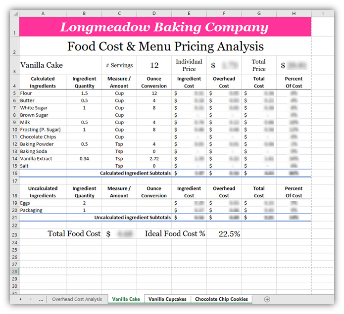
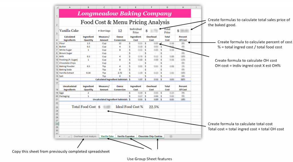
The completed spreadsheet should look like this:

Analyze Payment Options

1. Open your completed week 5 file (Food Cost Analysis workbook).
2. Select one (1) of the three recipe worksheets and:
   1. Move or Copy the worksheet,
   2. Create a Copy in a New Book
   3. Change the worksheet name to: Business Analysis
3. Close the Food Cost Analysis Workbook (do not save changes)
4. Edit the text in row 2 to read: Delivery Van (Lease vs. Purchase)
5. Delete Rows 3 to 23
6. You now have a workbook that has a consistent look to your previously created spreadsheets, but with no data. Save this workbook as “Business Analysis Workbook.xlsx”

7. You have researched the 3 different van prices. From the van dealer, you are able to get the price, yearly interest rate, the typical term of loan for purchase and lease, and the residual value for a lease. Enter the following information starting in Cell A4

8. Adjust formatting for each of the cells to make a good presentation (use wrap text and appropriately sized heights and widths of rows and columns)
9. Save your workbook before moving to the next section.

Editing and Creating the Business Analysis Worksheet

1. In cell F5 calculate the Monthly Payment for purchasing the vehicle using the PMT function
   1. Copy the Function to cells F6:F7

2. In cell G5, create a Formula to determine the total cost of the vehicle loan
   1. Copy the Formula to cells G6:G7

3. In cell F11, calculate the Monthly Payment for leasing the vehicle using the PMT function
   1. Copy the Function to cells F12:F13

4. In cell G11, create a Formula to determine the total cost of the vehicle lease over the life of the lease
   1. Copy the Formula to cells G12:G13

5. Starting In row 16, create a comparison table that shows:
   1. the 3 vans in column A – one van per row
   2. column B has the total Purchased monthly price – use a formula to connect the value that was calculated in Column F
   3. column C calculates your ⅓ share of the monthly purchase price
   4. column E has the total Lease monthly price – use a formula to connect the value that was calculated in Column F
   5. Column F calculates your ⅓ share of the monthly lease price

6. Use formatting to highlight the option that you recommend to your partners.
7. Format the worksheet and determine the best way to present your final work to the lender. Consider how you have formatted previous worksheets to make them more “professional” looking by using borders and cell styles.

**Save your workbook before continuing**

8. After bringing your analysis to your partners they asked if you could create a few charts that visually compare the vehicles by Monthly Payment and by Your Payment Portion to use for financing the delivery van with the lender.
9. Create a clustered column chart that best represents your partner’s request for a visual (chart) comparing the Monthly Purchase Payment vs. Monthly Lease Payment. Be sure to have the chart appear on a new sheet and be appropriately titled. Adjust the graph to:
   1. Edit the title to read: Monthly Purchase Payment vs. Monthly Lease Payment
   2. Increase the Font Size of the axis labels and legend to 12 point
   3. Be sure that the horizontal axis and vertical axis is properly labeled
   4. Change the Fill of the Monthly Lease Payment columns to #FF3399
10. Using the same information above create another similar chart to the Monthly Purchase Payment vs. Monthly Lease Payment chart you just made comparing the Partner Payment Portions (Purchase Payment and Lease Payments.) Be sure to have the chart appear on a new sheet and be appropriately titled. Adjust the graph to:
    1. Edit the title to read: Monthly Purchase Payment vs. Monthly Lease Payment
    2. Increase the Font Size of the axis labels and legend to 12 point
    3. Be sure that the horizontal axis and vertical axis is properly labeled
    4. Change the Fill of the Monthly Lease Payment columns to #FF3399
11. Save your workbook before submitting.

Congratulations!

You’ve worked hard to create realistic spreadsheets for the Longmeadow Baking Company.  You should be proud of all that you have accomplished.