Chapter 1
Section 1.2 – Entering, Editing, and Managing Data
Learning Objectives
-
Understand how to enter data into a worksheet.
-
Examine how to edit data in a worksheet.
-
Examine how Auto Fill is used when entering data.
-
Understand how to delete data from a worksheet and use the Undo command.
-
Examine how to adjust column widths and row heights in a worksheet.
In this section, we will begin the development of the workbook shown in Figure 1.1. The skills covered in this section are typically used in the early stages of developing one or more worksheets in a workbook.
Entering Data
You will begin building the workbook shown in Figure 1.1 by manually entering data into the worksheet. The following steps explain how the column headings in Row 2 are typed into the worksheet:
- Click cell location A2 on the worksheet.
- Type the word Month.
- Press the RIGHT ARROW key. This will enter the word into cell A2 and activate the next cell to the right.
- Type Unit Sales and press the RIGHT ARROW key.
- Repeat step 4 for the words Average Price and then again for Sales Dollars.
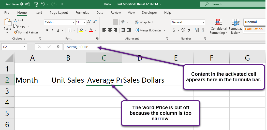
Figure 1.16 shows how your worksheet should appear after you have typed the column headings into Row 2. Notice that the word Price in cell location C2 is not visible. This is because the column is too narrow to fit the entry you typed. We will examine formatting techniques to correct this problem in the next section.
Integrity Check
Column Headings
It is critical to include column headings that accurately describe the data in each column of a worksheet. In professional environments, you will likely be sharing Excel workbooks with coworkers. Good column headings reduce the chance of someone misinterpreting the data contained in a worksheet, which could lead to costly errors depending on your career.
- Click cell location B3.
- Type the number 2670 and press the ENTER key. After you press the ENTER key, cell B4 will be activated. Using the ENTER key is an efficient way to enter data vertically down a column.
- Enter the following numbers in cells B4 through B14: 2160, 515, 590, 1030, 2875, 2700, 900, 775, 1180, 1800, and 3560.
- Click cell location C3.
- Type the number 9.99 and press the ENTER key.
- Enter the following numbers in cells C4 through C14: 12.49, 14.99, 17.49, 14.99, 12.49, 9.99, 19.99, 19.99, 19.99, 17.49, and 14.99.
- Activate cell location D3.
- Type the number 26685 and press the ENTER key.
- Enter the following numbers in cells D4 through D14: 26937, 7701, 10269, 15405, 35916, 26937, 17958, 15708, 23562, 31416, and 53370.
- When finished, check that the data you entered matches Figure 1.17.
Why?
Avoid Formatting Symbols When Entering Numbers
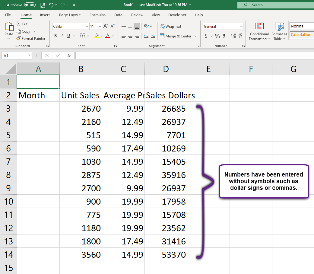
When typing numbers into an Excel worksheet, it is best to avoid adding any formatting symbols such as dollar signs and commas. Although Excel allows you to add these symbols while typing numbers, it slows down the process of entering data. It is more efficient to use Excel’s formatting features to add these symbols to numbers after you type them into a worksheet.
Integrity Check
Data Entry
It is very important to proofread your worksheet carefully, especially when you have entered numbers. Transposing numbers when entering data manually into a worksheet is a common error. For example, the number 563 could be transposed to 536. Such errors can seriously compromise the integrity of your workbook.
Figure 1.17 shows how your worksheet should appear after entering the data. Check your numbers carefully to make sure they are accurately entered into the worksheet.
Editing Data
Data that has been entered in a cell can be changed by double clicking the cell location or using the Formula Bar. You may have noticed that as you were typing data into a cell location, the data you typed appeared in the Formula Bar. The Formula Bar can be used for entering data into cells as well as for editing data that already exists in a cell. The following steps provide an example of entering and then editing data that has been entered into a cell location:
- Click cell A15 in the Sheet1 worksheet.
- Type the abbreviation Tot and press the ENTER key.
- Click cell A15.
- Move the mouse pointer up to the Formula Bar. You will see the pointer turn into a cursor. Move the cursor to the end of the abbreviation Tot and left click.
- Type the letters al to complete the word Total.
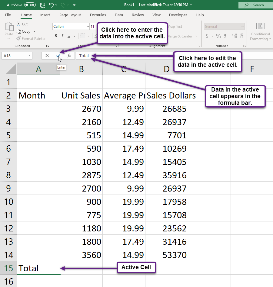
- Click the checkmark to the left of the Formula Bar (see Figure 1.18). This will enter the change into the cell.
- Double click cell A15.
- Add a space after the word Total and type the word Sales.
- Press the ENTER key.
Keyboard Shortcuts
Editing Data in a Cell
Activate the cell that is to be edited and press the F2 key on your keyboard.
Auto Fill
The Auto Fill feature is a valuable tool when manually entering data into a worksheet. This feature has many uses, but it is most beneficial when you are entering data in a defined sequence, such as the numbers 2, 4, 6, 8, and so on, or nonnumeric data such as the days of the week or months of the year. The following steps demonstrate how Auto Fill can be used to enter the months of the year in Column A:
- Click cell A3 in the Sheet1 worksheet.
- Type the word January and press the ENTER key.
- Activate cell A3 again.
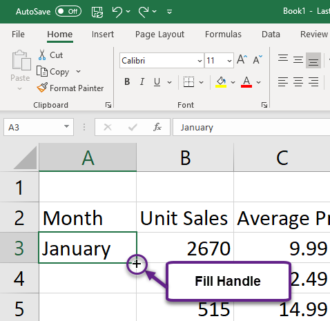
- Move the mouse pointer to the lower right corner of cell A3. You will see a small square in this corner of the cell; this is called the Fill Handle (See Figure 1.19) When the mouse pointer gets close to the Fill Handle, the white block plus sign will turn into a black plus sign.
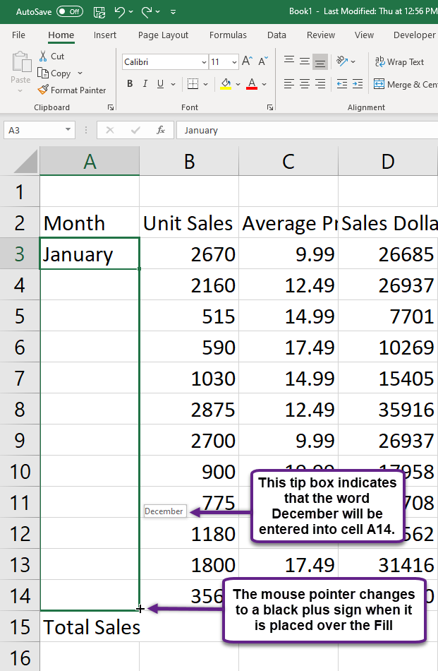
Left click and drag the Fill Handle to cell A14. Notice that the Auto Fill tip box indicates what month will be placed into each cell (see Figure 1.20). Release the left mouse button when the tip box reads “December.”
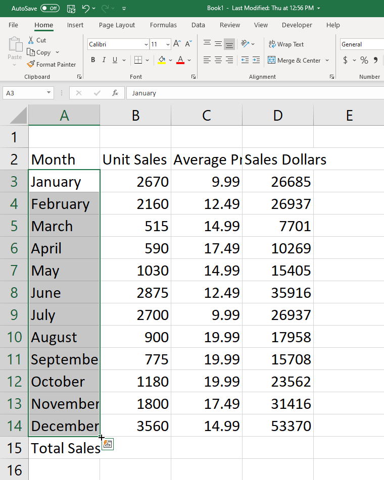
Once you release the left mouse button, all twelve months of the year should appear in the cell range A3:A14, as shown in Figure 1.21.
Deleting Data and the Undo Command
There are several methods for removing data from a worksheet, a few of which are demonstrated here. With each method, you use the Undo command. This is a helpful command in the event you mistakenly remove data from your worksheet. The following steps demonstrate how you can delete data from a cell or range of cells:
- Click cell C2 by placing the mouse pointer over the cell and clicking the left mouse button.
- Press the DELETE key on your keyboard. This removes the contents of the cell.
- Highlight the range C3:C14 by placing the mouse pointer over cell C3. Then left click and drag the mouse pointer down to cell C14.
- Place the mouse pointer over the Fill Handle. You will see the white block plus sign change to a black plus sign.
- Click and drag the mouse pointer up to cell C3 (see Figure 1.22). Release the mouse button. The contents in the range C3:C14 will be removed.
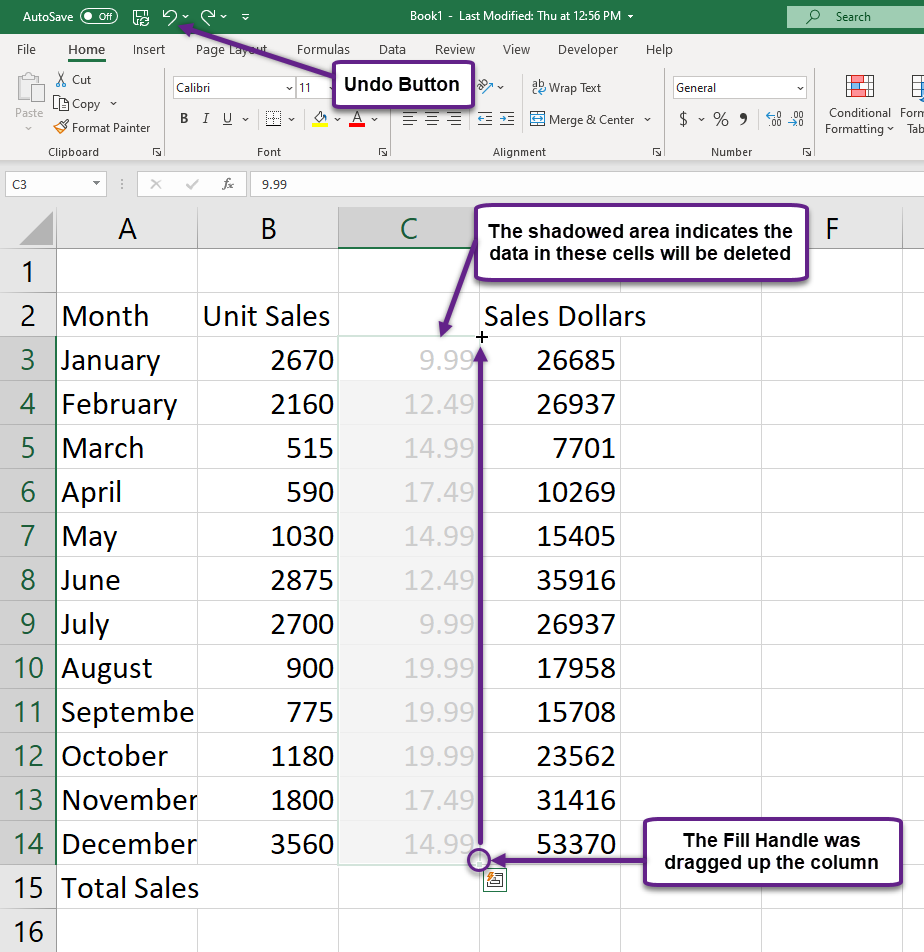
- Click the Undo button in the Quick Access Toolbar (see Figure 1.22). This should replace the data in the range C3:C14.
- Click the Undo button again. This should replace the data in cell C2.
Keyboard Shortcuts
Undo Command:
- Hold down the CTRL key while pressing the letter Z on your keyboard.
- Highlight the range C2:C14 by placing the mouse pointer over cell C2. Then left click and drag the mouse pointer down to cell C14.
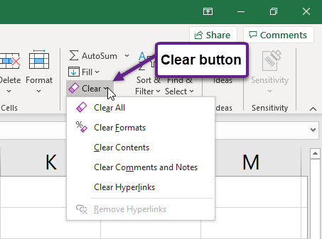
- Click the Clear button in the Home tab of the Ribbon, which is next to the Cells group of commands (see Figure 1.23). This opens a drop-down menu that contains several options for removing or clearing data from a cell. Notice that you also have options for clearing just the formats in a cell or the hyperlinks in a cell.
- Click the Clear All option. This removes the data in the cell range.
- Click the Undo button. This replaces the data in the range C2:C14.
Adjusting Columns and Rows
There are a few entries in the worksheet that appear cut off. For example, the last letter of the word September cannot be seen in cell A11. This is because the column is too narrow for this word. The columns and rows on an Excel worksheet can be adjusted to accommodate the data that is being entered into a cell. The following steps explain how to adjust the column widths and row heights in a worksheet:
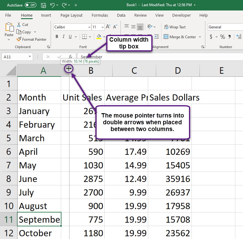
- Bring the mouse pointer between Column A and Column B in the Sheet1 worksheet, as shown in Figure 1.24. You will see the white block plus sign turn into double arrows.
- Click and drag the column to the right so the entire word September in cell A11 can be seen. As you drag the column, you will see the column width tip box. This box displays the number of characters that will fit into the column using the Calibri 11-point font which is the default setting for font/size.
- Release the left mouse button.
You may find that using the click-and-drag method is inefficient if you need to set a specific character width for one or more columns. Steps 1 through 6 illustrate a second method for adjusting column widths when using a specific number of characters:
- Click any cell location in Column A by moving the mouse pointer over a cell location and clicking the left mouse button. You can highlight cell locations in multiple columns if you are setting the same character width for more than one column.
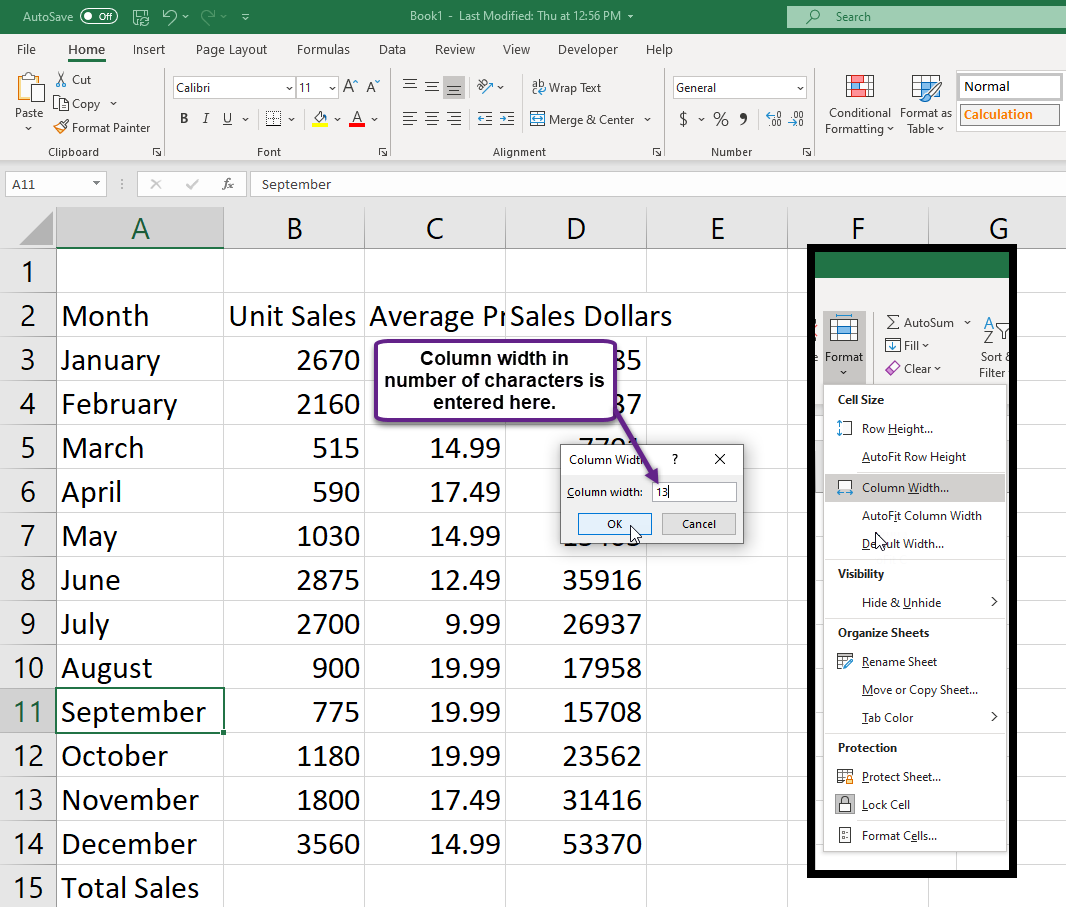
- In the Home tab of the Ribbon, left click the Format button in the Cells group.
- Click the Column Width option from the drop-down menu. This will open the Column Width dialog box.
- Type the number 13 and click the OK button on the Column Width dialog box. This will set Column A to this character width (see Figure 1.25).
- Once again bring the mouse pointer between Column A and Column B so that the double arrow pointer displays and then double-click to activate AutoFit. This feature adjusts the column width based on the longest entry in the column.
- Use the Column Width dialog box (step 6 above) to reset the width to 13.
Keyboard Shortcuts
Column Width
Press the ALT key on your keyboard, then press the letters H, O, and W one at a time.
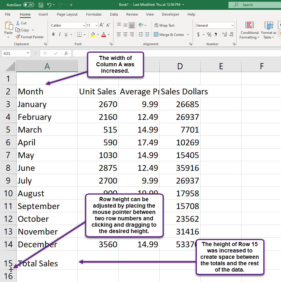
Steps 1 through 4 demonstrate how to adjust row height, which is similar to adjusting column width:
- Click cell A15 by placing the mouse pointer over the cell and clicking the left mouse button.
- In the Home tab of the Ribbon, left click the Format button in the Cells group.
- Click the Row Height option from the drop-down menu. This will open the Row Height dialog box.
- Type the number 24 and click the OK button on the Row Height dialog box. This will set Row 15 to a height of 24 points. A point is equivalent to approximately 1/72 of an inch. This adjustment in row height was made to create space between the totals for this worksheet and the rest of the data.
Keyboard Shortcuts
Row Height
- Press the ALT key on your keyboard, then press the letters H, O, and H one at a time.
Figure 1.26 shows the appearance of the worksheet after Column A and Row 15 are adjusted:
Skill Refresher
Adjusting Columns and Rows
- Activate at least one cell in the row or column you are adjusting.
- Click the Home tab of the Ribbon.
- Click the Format button in the Cells group.
- Click either Row Height or Column Width from the drop-down menu.
- Enter the Row Height in points or Column Width in characters in the dialog box.
- Click the OK button.
Key Takeaways
- Column headings should be used in a worksheet and should accurately describe the data contained in each column.
- Using symbols such as dollar signs when entering numbers into a worksheet can slow down the data entry process.
- Worksheets must be carefully proofread when data has been manually entered.
- The Undo command is a valuable tool for recovering data that was deleted from a worksheet.
