This section addresses formatting commands that can be used to enhance the visual appearance of a worksheet. It also provides an introduction to mathematical calculations. The skills introduced in this section will give you powerful tools for analyzing the data that we have been working with in this workbook and will highlight how Excel is used to make key decisions in virtually any career. Additionally, Excel Spreadsheet Guidelines for format and appearance will be introduced as a format for the course and spreadsheets submitted.

Formatting Data and Cells

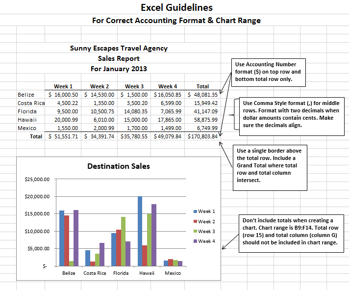
Enhancing the visual appearance of a worksheet is a critical step in creating a valuable tool for you or your coworkers when making key decisions. There are accepted professional formatting standards when spreadsheets contain only currency data. For this course, we will use the following Excel Guidelines for Formatting. The first figure displays how to use Accounting number format when ALL figures are currency. Only the first row of data and the totals should be formatted with the Accounting format.  The other data should be formatted with Comma style.  There also needs to be a Top Border above the numbers in the total row.  If any of the numbers have cents, you need to format all of the data with two decimal places.

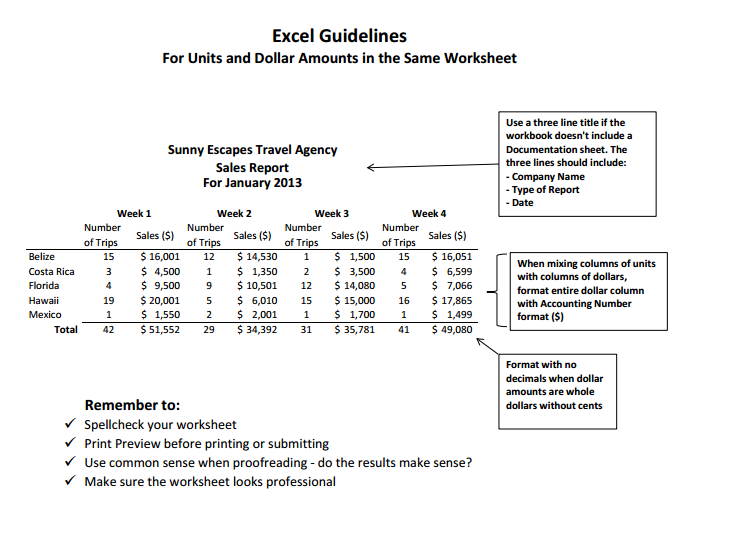
Often, your Excel spreadsheet will contain values that are both currency and non-currency in nature. When that is the case, you will want to use the guidelines in the following figure:

The following steps demonstrate several fundamental formatting skills that will be applied to the workbook that we are developing for this chapter. Several of these formatting skills are identical to ones that you may have already used in other Microsoft applications such as Microsoft® Word® or Microsoft® PowerPoint®.

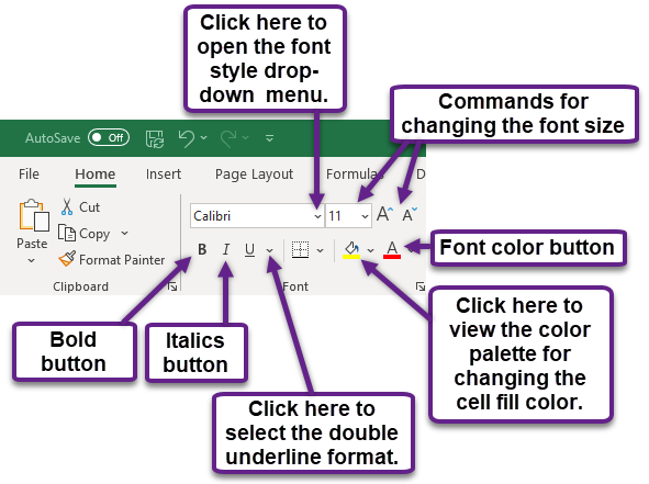
1. Highlight the range A2:D2 in the Sheet1 worksheet by placing the mouse pointer over cell A2 and left clicking and dragging to cell D2. Click the Bold button in the Font group of commands in the Home tab of the ribbon.
2. Click the Border button in the Font group of commands in the Home tab of the Ribbon (see Figure 1.32). Select the Bottom Border option from the list to achieve the goal of a border on the bottom of row 2 below the column headings.

3. Highlight the range A15:D15 by placing the mouse pointer over cell A15 and left clicking and dragging to cell D15.
4. Click the Bold button in the Font group of commands in the Home tab of the Ribbon.
5. Click the Border button in the Font group of commands in the Home tab of the Ribbon (see Figure 1.32). Select the Top Border option from the list to achieve the goal of a border on the top of row 15 where totals will eventually display.\

6. Highlight the range B3:B14 by placing the mouse pointer over cell B3 and left clicking and dragging down to cell B14.
7. Click the Comma Style button in the Number group of commands in the Home tab of the Ribbon. This feature adds a comma as well as two decimal places. (see Figure 1.33).

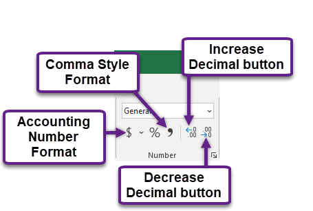
8. Since the figures in this range do not include cents, click the Decrease Decimal button in the Number group of commands in the Home tab of the Ribbon two times (see Figure 1.33).
9. The numbers will also be reduced to zero decimal places.
10. Highlight the range C3:C14 by placing the mouse pointer over cell C3 and left clicking and dragging down to cell C14.
11. Click the Accounting Number Format button in the Number group of commands in the Home tab of the Ribbon (see Figure 1.33). This will add the US currency symbol and two decimal places to the values. This format is common when working with pricing data. As discussed above in the Formatting Data and Cells section, you will want to use Accounting format on all values in this range since the worksheet contains non-currency as well as currency data.
12. Highlight the range D3:D14 by placing the mouse pointer over cell D3 and left clicking and dragging down to cell D14.
13. Again, select the Accounting Number Format; this will add the US currency symbol to the values as well as two decimal places.
14. Click the Decrease Decimal button in the Number group of commands in the Home tab of the Ribbon.
15. This will add the US currency symbol to the values and reduce the decimal places to zero since there are no cents in these figures.
16. Highlight the range A1:D1 by placing the mouse pointer over cell A1 and left clicking and dragging over to cell D1.
17. Click the down arrow next to the Fill Color button in the Font group of commands in the Home tab of the Ribbon (see Figure 1.34). This will prepare the range for a worksheet title.

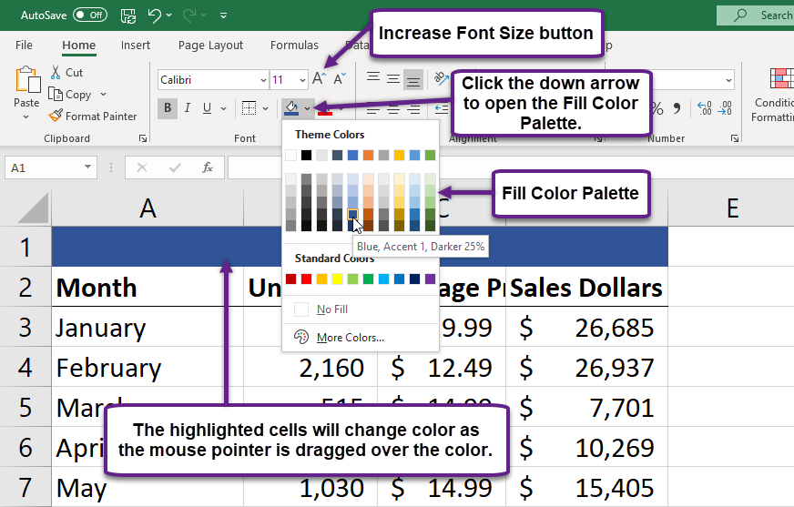
18. Click the Blue, Accent 1, Darker 25% color from the palette (see Figure 1.34). Notice that as you move the mouse pointer over the color palette, you will see a preview of how the color will appear in the highlighted cells. Experiment with this feature.
19. Click on A1 and enter the worksheet title: General Merchandise World and click on the check mark in the formula bar to enter this information.
20. Since the black font is difficult to read on the blue background, you’ll change the font color to be more visible. Click the down arrow next to the Font Color button in the Font group of commands in the Home tab of the Ribbon; select White as the font color for this range (see Figure 1.32).
21. Highlight the range A1:D1 by placing the mouse pointer over cell A1 and and dragging across to cell D1.
22. Click the drop-down arrow on the right side of the Font button in the Home tab of the Ribbon; select Arial as the font for this range. (see Figure 1.32).
23. Notice that as you move the mouse pointer over the font style options, you can see the font change in the highlighted cells.
24. Expand the column width of Column D to 14 characters.

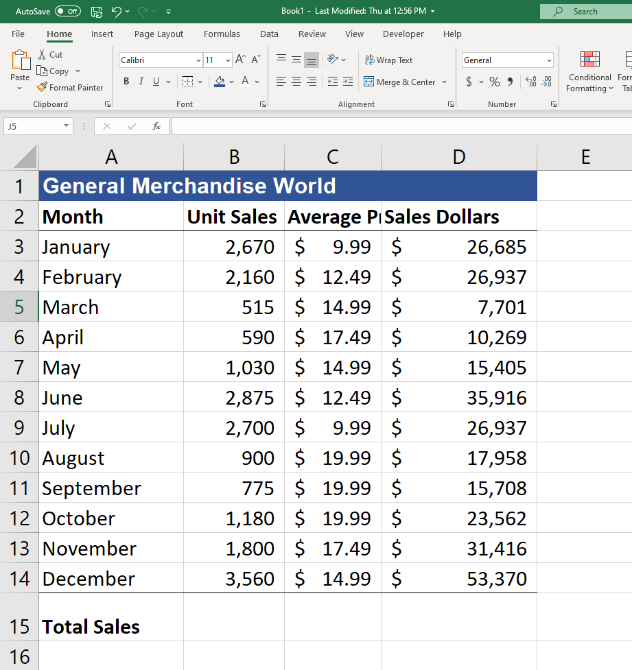
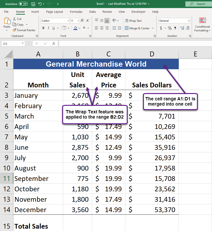
Figure 1.35 shows how the Sheet1 worksheet should appear after the formatting techniques are applied:

Data Alignment (Wrap Text, Merge Cells, and Center)

The skills presented in this segment show how data are aligned within cell locations. For example, text and numbers can be centered in a cell location, left justified, right justified, and so on. In some cases you may want to stack multiword text entries vertically in a cell instead of expanding the width of a column. This is referred to as wrapping text. These skills are demonstrated in the following steps:

1. Highlight the range B2:D2 by placing the mouse pointer over cell B2 and left clicking and dragging over to cell D2.
2. Click the Center button in the Alignment group of commands in the Home tab of the Ribbon (see Figure 1.36). This will center the column headings in each cell location.

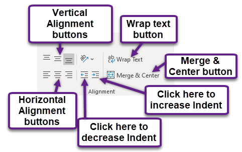
3. Click the Wrap Text button in the Alignment group (see Figure 1.36). The height of Row 2 automatically expands, and the words that were cut off because the columns were too narrow are now stacked vertically.

4. Highlight the range A1:D1 by placing the mouse pointer over cell A1 and left clicking and dragging over to cell D1.
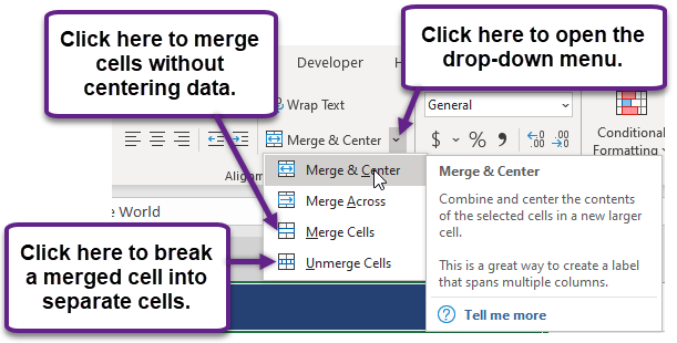
5. Click the down arrow on the right side of the Merge & Center button in the Alignment group of commands in the Home tab of the Ribbon.
6. Left click the Merge & Center option (see Figure 1.37). This will create one large cell location running across the top of the data set.

Figure 1.38 shows the Sheet1 worksheet with the data alignment commands applied. The reason for merging the cells in the range A1:D1 will become apparent in the next segment.

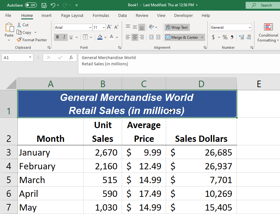
Entering Multiple Lines of Text

In the Sheet1 worksheet, the cells in the range A1:D1 were merged for the purposes of adding a title to the worksheet. This worksheet will contain both a title and a subtitle. The following steps explain how you can enter text into a cell and determine where you want the second line of text to begin:

1. Activate cell A1 in the Sheet1 worksheet by placing the mouse pointer over cell A1 and clicking the left mouse button. Since the cells were merged, clicking cell A1 will automatically activate the range A1:D1. Position your mouse to the end of the title, directly after the “d” in the word “World” and double-click to get a cursor (flashing I-beam).
2. Hold down the ALT key and press the ENTER key. This will start a new line of text in this cell location.
3. Type the text Retail Sales (in millions) and press the ENTER key.
4. Select cell A1. Then click the Italics and Bold buttons in the Font group of commands in the Home tab of the Ribbon.
5. Increase the height of Row 1 to 30 points. Once the row height is increased, all the text typed into the cell will be visible (see Figure 1.39).

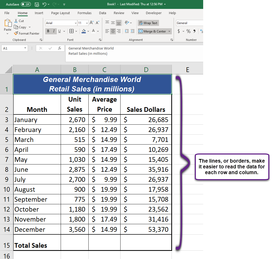
Borders (Adding Lines to a Worksheet)

In Excel, adding custom lines to a worksheet is known as adding borders. Borders are different from the grid lines that appear on a worksheet and that define the perimeter of the cell locations. The Borders command lets you add a variety of line styles to a worksheet that can make reading the worksheet much easier. The following steps illustrate methods for adding preset borders and custom borders to a worksheet:

1. Click the down arrow to the right of the Borders button in the Font group of commands in the Home page of the Ribbon to view border options. (see Figure 1.40).

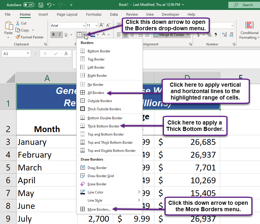
2. Highlight the range A1:D15. Left click the All Borders option from the Borders drop-down menu (see Figure 1.40). This will add vertical and horizontal lines to the range A1:D15.
3. Highlight the range A2:D2 by placing the mouse pointer over cell A2 and left clicking and dragging over to cell D2.
4. Click the down arrow to the right of the Borders button.
5. Left click the Thick Bottom Border option from the Borders drop-down menu.
6. Highlight the range A14:D14 and apply a Thick Bottom Border from the drop-down menu. The thick border will help maintain the Excel Formatting Guidelines.
7. Highlight the range A1:D15.
8. Click the down arrow to the right of the Borders button.
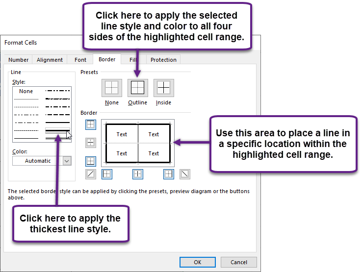
9. Click More Borders… at the bottom of the List.
10. This will open the Format Cells dialog box (see Figure 1.41). You can access all formatting commands in Excel through this dialog box.
11. In the Style section of the Borders tab, left click the thickest line style (see Figure 1.41).
12. Left click the Outline button in the Presets section (see Figure 1.41).
13. Click the OK button at the bottom of the dialog box (see Figure 1.41).

AutoSum

You will see at the bottom of Figure 1.42 that Row 15 is intended to show the totals for the data in this worksheet. Applying mathematical computations to a range of cells is accomplished through functions in Excel. Chapter 2 “Mathematical Computations” will review mathematical formulas and functions in detail. However, the following steps will demonstrate how you can quickly sum the values in a column of data using the AutoSum command:

1. Activate cell B15 in the Sheet1 worksheet.
2. Click the Formulas tab of the Ribbon.
3. Click the down arrow below the AutoSum button in the Function Library group of commands (see Figure 1.43). Note that the AutoSum button can also be found in the Editing group of commands in the Home tab of the Ribbon.

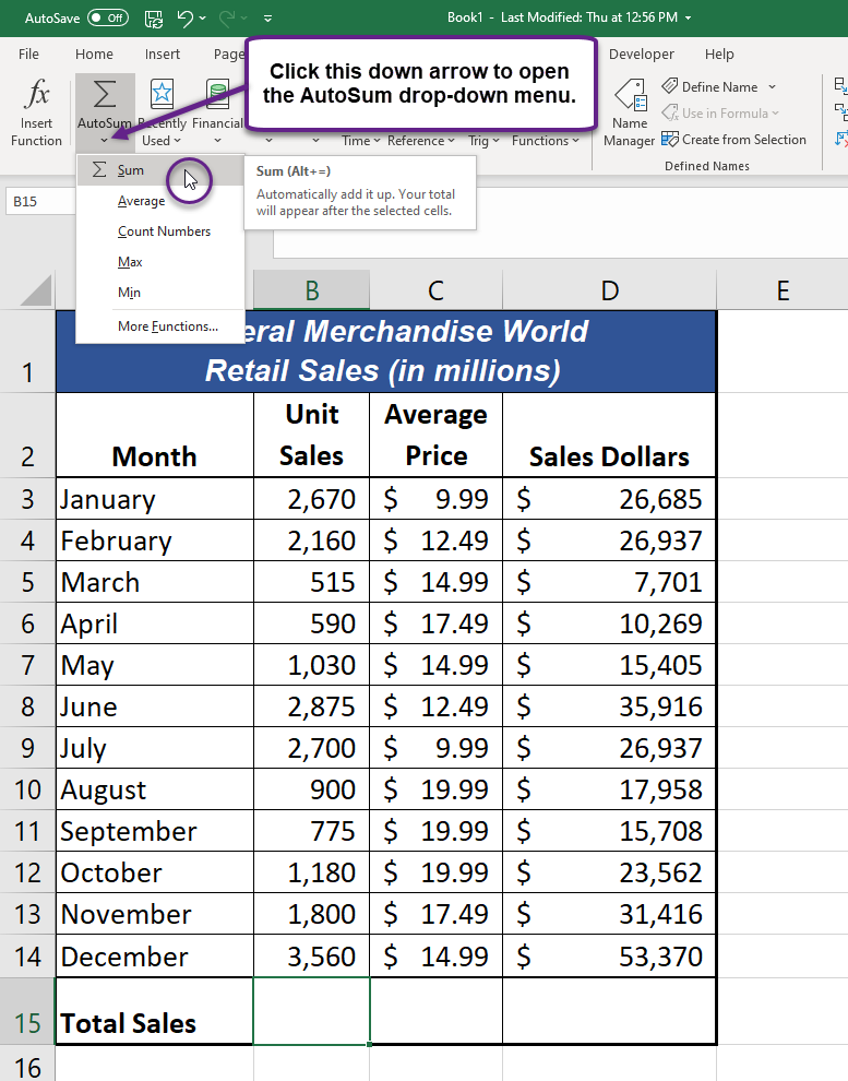
4. Click the Sum option from the AutoSum drop-down menu. The first click will display a flashing marquee around the range. Click the check mark next to the Formula bar to complete the function.
5. Excel will provide a total for the values in the Unit Sales column.
6. Activate cell D15. It would not make sense to total the averages in column C so C15 will be left blank.
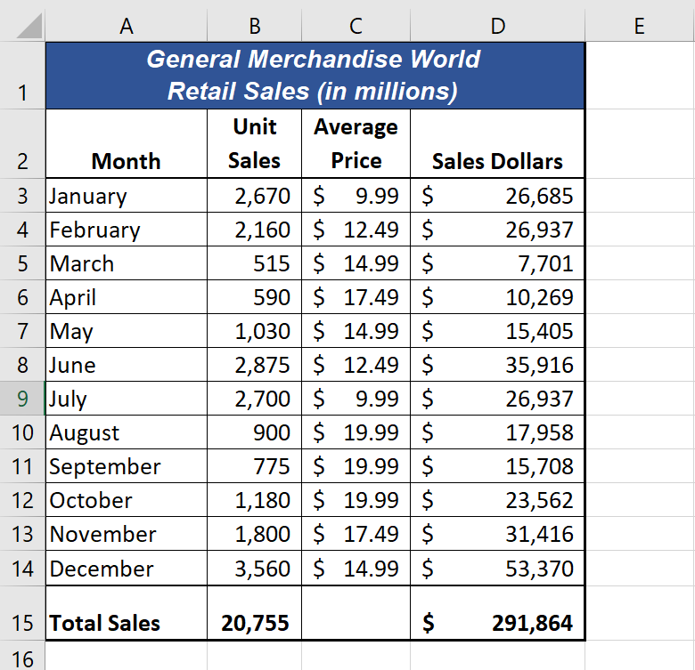
7. Repeat steps 3 through 5 to sum the values in the Sales Dollars column (see Figure 1.44).

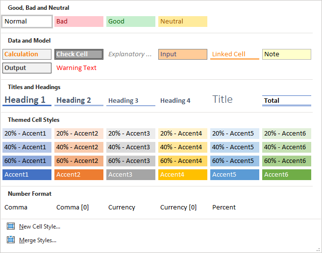
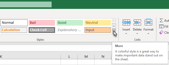
Cell Styles Menu

Cell styles allow you to apply several formats to data in one step, which allows for consistent formatting. The cell style has a pre-defined set of formatting that are associated with the document theme, which include the fonts, borders, and shading. There are several built-in cell styles to choose from to format data (see Figure 1.45).

To apply a cell style:

1. select the cells, data, columns, or rows you want to format
2. On the Home tab, in the Styles group click the More dropdown arrow (see Figure 1.46)
3. Select a cell style and click on it to apply it