Chapter 3
Section 3.1 – More on Formulas and Functions
FILE: CH 3.1
The AVERAGE Function
The next function we will add to the Budget Detail worksheet is the AVERAGE function. This function is used to calculate the arithmetic mean for a group of numbers. For the Budget Detail worksheet, we will use the function to calculate the average of the values in the Annual Spend column. We will add this to the worksheet by using the Function Library. The following steps explain how this is accomplished:
- Click cell D14 in the Budget Detail worksheet.
- Click the Formulas tab on the Ribbon.
- Click the More Functions button in the Function Library group of commands.
- Place the mouse pointer over the Statistical option from the drop-down list of options.
- Click the AVERAGE function name from the list of functions that appear in the menu (see Figure 3.1). This opens the Function Arguments dialog box.
- Click the Collapse Dialog button in the Function Arguments dialog box (see Figure 3.2).
- Highlight the range D3:D11.
- Click the Expand Dialog button in the Function Arguments dialog box (see Figure 3.3). You can also press the ENTER key to get the same result.
- Click the OK button on the Function Arguments dialog box. This adds the AVERAGE function to the worksheet.
Figure 3.1 illustrates how a function is selected from the Function Library in the Formulas tab of the Ribbon:
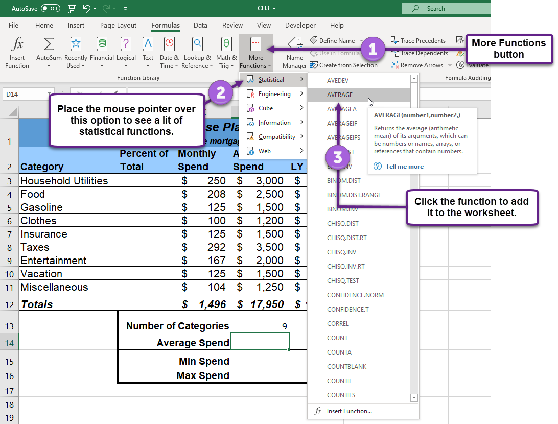
Figure 3.2 shows the Function Arguments dialog box. This appears after a function is selected from the Function Library. The Collapse Dialog button is used to hide the dialog box so a range of cells can be highlighted on the worksheet and then added to the function.
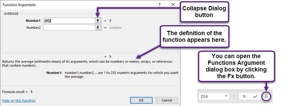
Figure 3.3 shows how a range of cells can be selected from the Function Arguments dialog box once it has been collapsed.
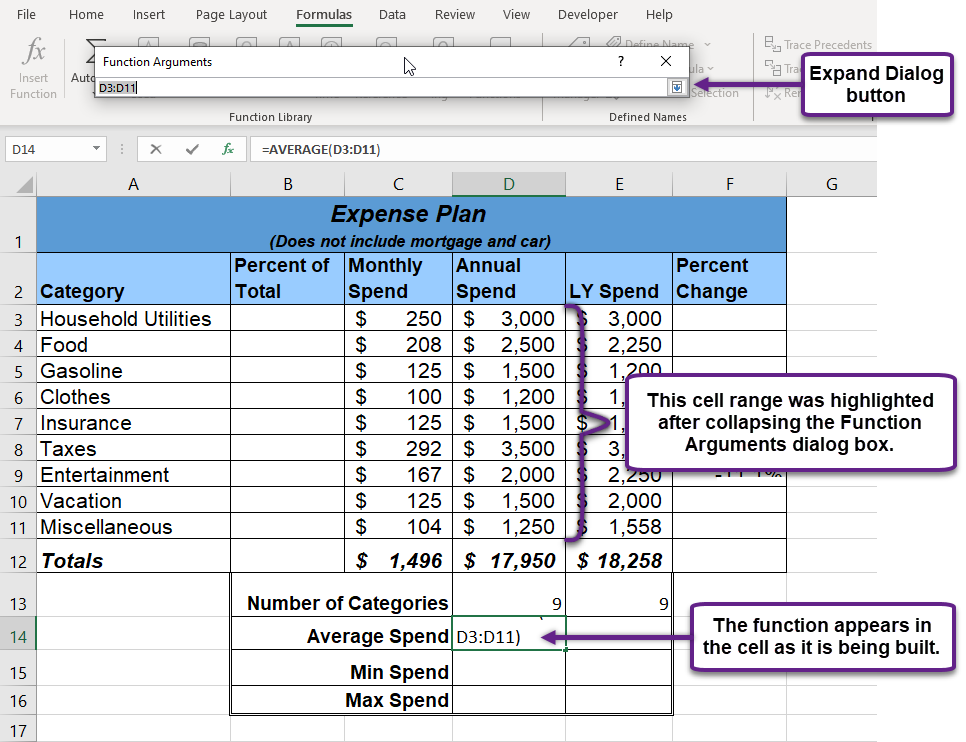
Figure 3.4 shows the Function Arguments dialog box after the cell range is defined for the AVERAGE function. The dialog box shows the result of the function before it is added to the cell location. This allows you to assess the function output to determine whether it makes sense before adding it to the worksheet.
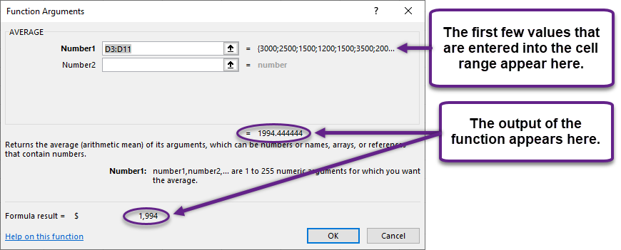
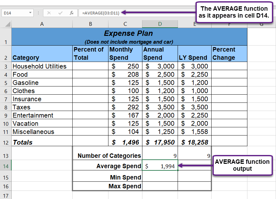
Figure 3.5 shows the completed AVERAGE function in the Budget Detail worksheet. The output of the function shows that on average we expect to spend $1,994 for each of the categories listed in Column A of the budget. This average spend calculation per category can be used as an indicator to determine which categories are costing more or less than the average budgeted spend dollars.
The MAX and MIN Functions
The final two statistical functions that we will add to the Budget Detail worksheet are the MAX and MIN functions. These functions identify the highest and lowest values in a range of cells. The following steps explain how to add these functions to the Budget Detail worksheet:
- Click cell D15 in the Budget Detail worksheet.
- Type an equal sign =.
- Type the word MIN.
- Type an open parenthesis (.
- Highlight the range D3:D11.
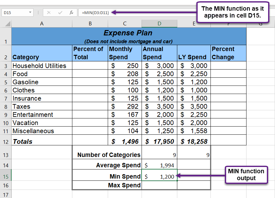
- Type a closing parenthesis ) and press the ENTER key, or simply press the ENTER key and Excel will close the function for you. The MIN function produces an output of $1,200, which is the lowest value in the Annual Spend column (see Figure 3.6).
- Click cell D16.
- Type an equal sign =.
- Type the word MAX.
- Type an open parenthesis (.
- Highlight the range D3:D11.
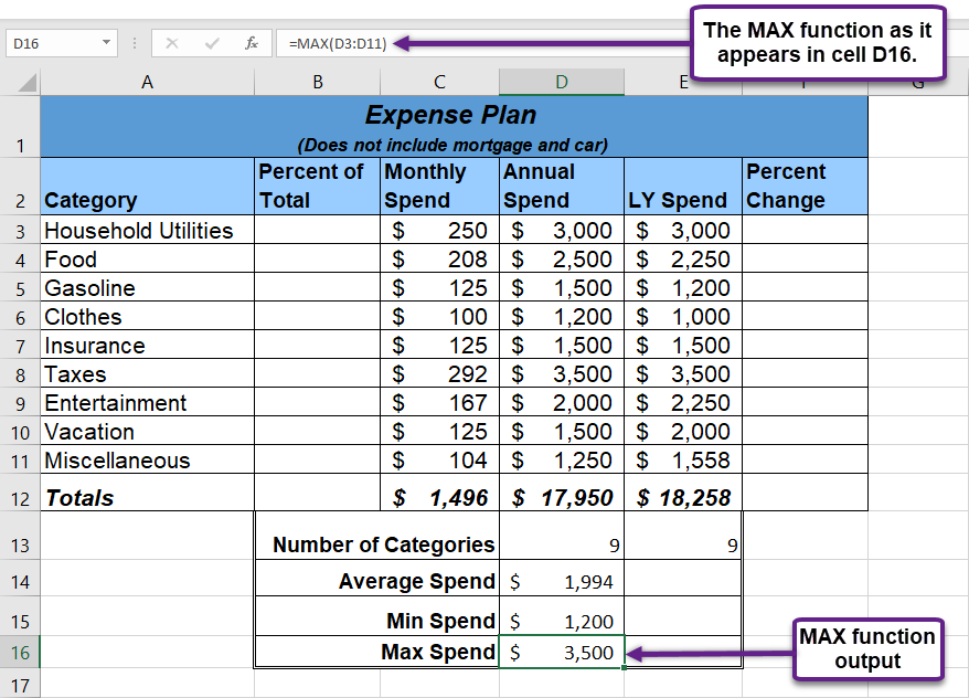
- Type a closing parenthesis ) and press the ENTER key, or simply press the ENTER key and Excel will close the function for you. The MAX function produces an output of $3,500. This is the highest value in the Annual Spend column (see Figure 3.7).
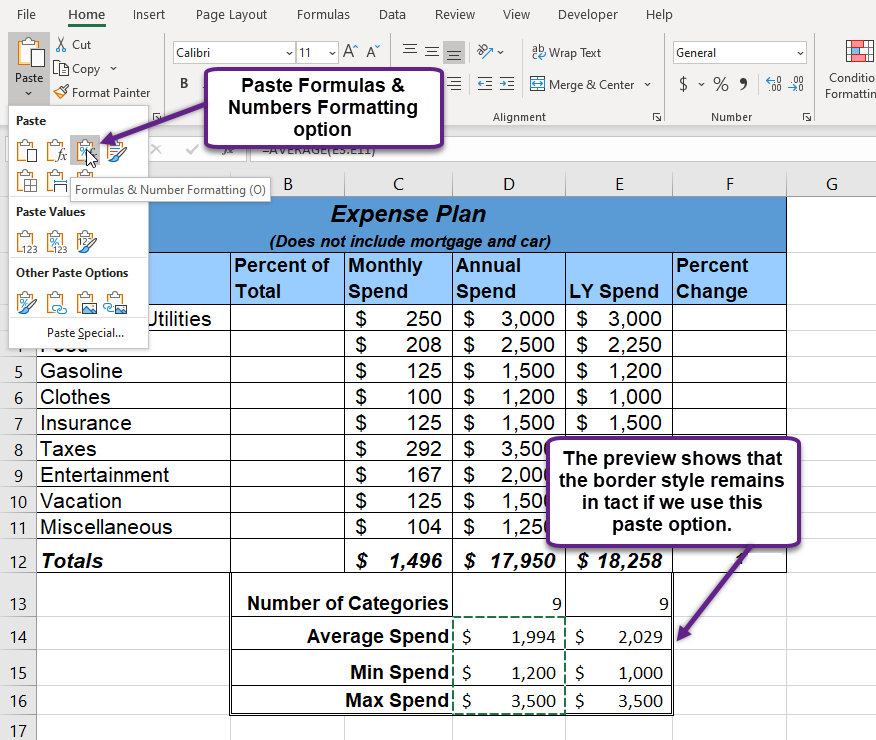
- Copy the functions from cells D14:D16 to cells E14:E16 using the Paste Formulas & Number Formatting option in the Paste drop-down menu while maintaining the double border style (see Figure 3.8).
Skill Refresher
Statistical Functions:
- Type an equal sign =.
- Type the function name followed by an open parenthesis ( or double click the function name from the function list.
- Highlight a range on a worksheet or click individual cell locations followed by commas.
- Type a closing parenthesis ) and press the ENTER key or press the ENTER key to close the function.
