Download and open File: CH 2.2

Inserting Columns and Rows

Using Excel workbooks that have been created by others is a very efficient way to work because it eliminates the need to create data worksheets from scratch. However, you may find that to accomplish your goals, you need to add additional columns or rows of data. In this case, you can insert blank columns or rows into a worksheet. The following steps demonstrate how to do this:

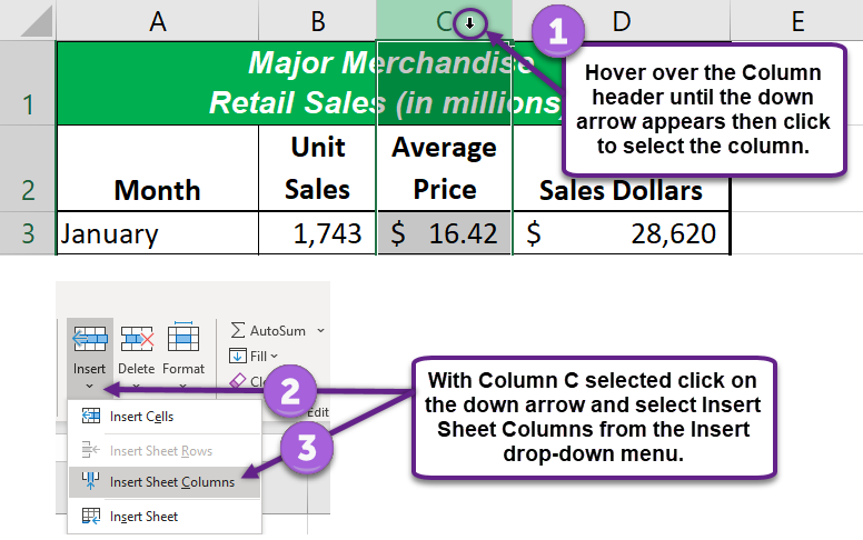
1. Click Column C in the worksheet by placing the mouse pointer over the column header location until you see a bold down arrow and click the left mouse button to select the column (see Figure 2.15).
2. Click the down arrow on the Insert button in the Home tab of the Ribbon (see Figure 2.15).
3. Click the Insert Sheet Columns option from the drop-down menu (see Figure 2.15). A blank column will be inserted to the left of Column C. The contents that were previously in Column C now appear in Column D. Note that columns are always inserted to the left of the activated cell.

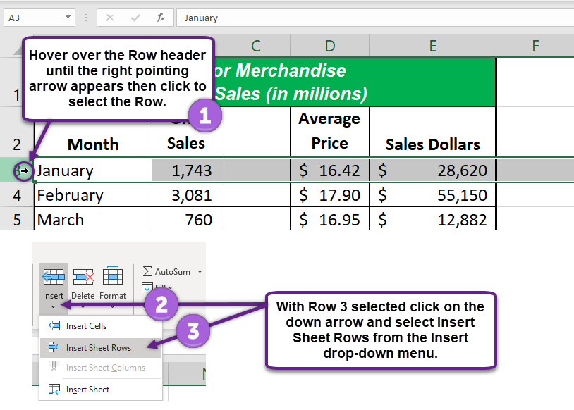
1. Click Row 3 in the CH2.2 worksheet by placing the mouse pointer over the Row header and clicking the left mouse button.
2. Click the down arrow on the Insert button in the Home tab of the Ribbon (see Figure 2.16).
3. Click the Insert Sheet Rows option from the drop-down menu (see Figure 2.16). A blank row will be inserted above Row 3. The contents that were previously in Row 3 now appear in Row 4. Note that rows are always inserted above the activated cell.

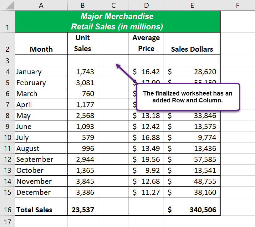
Your completed work should look like Figure 2.17 seen below.

Deleting Columns and Rows

You may need to delete entire columns or rows of data from a worksheet. This need may arise if you need to remove either blank columns or rows from a worksheet or columns and rows that contain data. The methods for removing cell contents were covered earlier and can be used to delete unwanted data. However, if you do not want a blank row or column in your workbook, you can delete it using the following steps:

1. Click cell C3 by placing the mouse pointer over the cell location and clicking the left mouse button.
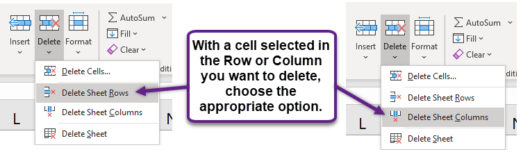
2. Click the down arrow on the Delete button in the Cells group in the Home tab of the Ribbon.
3. Click the Delete Sheet Rows option from the drop-down menu (see Figure 2.18). This removes Row 3 and shifts all the data (below Row 2) in the worksheet up one row.

4. Click cell C3 by placing the mouse pointer over the cell location and clicking the left mouse button.
5. Click the down arrow on the Delete button in the Cells group in the Home tab of the Ribbon.
6. Click the Delete Sheet Columns option from the drop-down menu (see Figure 2.18). This removes Column C and shifts all the data in the worksheet (to the right of Column B) over one column to the left.
7. After deleting Column C and Row 3 your work should resemble Figure 2.19.
8. Save the changes to your workbook by clicking either the Save button on the Home ribbon; or by selecting the Save option from the File menu.

Moving Data

Once data are entered into a worksheet, you can move it to different locations. The following steps demonstrate how to move data to different locations on a worksheet:

1. Select Column C on the CH2.2 workbook and insert a new column.
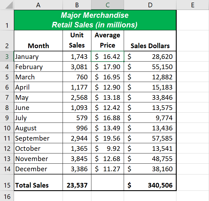
2. Highlight the range D2:D15 by activating cell D2 and clicking and dragging down to cell D15.
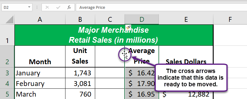
3. Bring the mouse pointer to the left edge of cell D2. You will see the white block plus sign change to cross arrows (see Figure 2.20). This indicates that you can left click and drag the data to a new location.

4. Left Click and drag the mouse pointer to cell C2.
5. Release the left mouse button. The data now appears in Column C.
6. Click the Undo button in the Quick Access Toolbar. This moves the data back to Column D.

The Format Painter

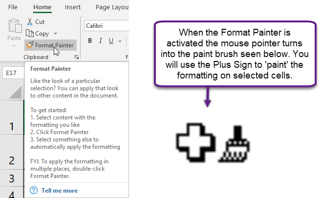
The Format Painter on the Home tab allows the application of ALL the formatting of one cell(s) to others (see Figure 2.21). The formats it will copy include fonts, colors, size, borders, and text. The Format Painter will copy ALL the formatting of a cell(s) and paste it to the selected cell(s).

1. Select cell A2.
2. Click on the Format Painter button on the Home tab (see Figure 2.21).
3. Using the Plus Sign mouse pointer select the cell range A3:A14.
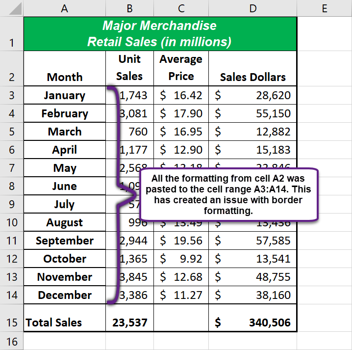
4. This will copy ALL the formatting of cell A2 to the cell range A3:A14 (see Figure 2.22).

Note that the cell formatting, alignment, and font style all changed, which altered the appearance of your worksheet negatively. Be careful when you choose to use this tool.