Chapter 2
Section 2.2 – Statistical Functions
Learning Objectives
- Use the SUM function to calculate totals.
- Use absolute references to calculate percent of totals.
- Use the COUNT function to count cell locations with numerical values.
- Use the COUNTA function to count cell locations with numeric and text values.
In addition to formulas, another way to conduct mathematical computations in Excel is through functions. Statistical functions apply a mathematical process to a group of cells in a worksheet. For example, the SUM function is used to add the values contained in a range of cells. A list of commonly used statistical functions is shown in Table 2.4. Functions are more efficient than formulas when you are applying a mathematical process to a group of cells. If you use a formula to add the values in a range of cells, you will have to add each cell location to the formula one at a time. This can be very time-consuming if you must add the values in a few hundred cell locations. However, when you use a function, you can highlight all the cells that contain values you wish to sum in just one step. This section demonstrates a variety of statistical functions that we will add to the Personal Budget workbook. In addition to demonstrating functions, this section also reviews percent of total calculations and the use of absolute references.
Continue using File: CH 2.1
Table 2.3 – Commonly Used Statistical Functions |
||
Function |
Output |
|
|
AVERAGE |
The average or arithmetic mean for a group of numbers |
|
|
COUNT |
The number of cell locations in a range that contain a numeric character |
|
|
COUNTA |
The number of cell locations in a range that contain a text or numeric character |
|
|
MAX |
The highest numeric value in a group of numbers |
|
|
MIN |
The lowest numeric value in a group of numbers |
|
|
SUM |
The total of all numeric values in a group |
|
The SUM Function
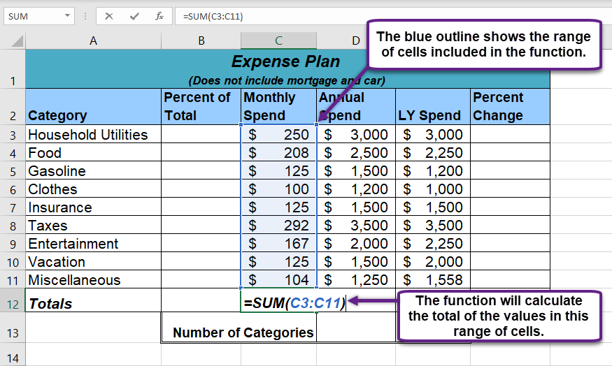
The SUM function is used when you need to calculate totals for a range of cells or a group of selected cells on a worksheet. With regard to the Budget Detail worksheet, we will use the SUM function to calculate the totals in row 12. It is important to note that there are several methods for adding a function to a worksheet, which will be demonstrated throughout the remainder of this chapter. The following illustrates how a function can be added to a worksheet by typing it into a cell location:
- Click the Budget Detail worksheet tab to open the worksheet.
- Click cell C12.
- Type an equal sign =.
- Type the function name SUM.
- Type an open parenthesis (.
- Click cell C3 and drag down to cell C11. This places the range C3:C11 into the function.
- Type a closing parenthesis).
- Press the ENTER key. The function calculates the total for the Monthly Spend column, which is $1,496.
Figure 2.6 shows the appearance of the SUM function added to the Budget Detail worksheet before pressing the ENTER key.
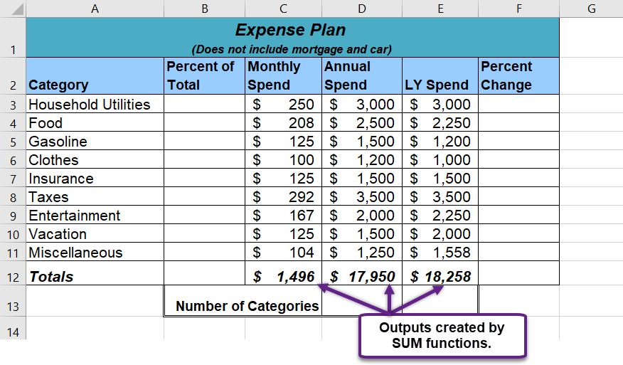
As shown in Figure 2.6, the SUM function was added to cell C12. However, this function is also needed to calculate the totals in the Annual Spend and LY Spend columns. The function can be copied and pasted into these cell locations because of relative referencing. Relative referencing serves the same purpose for functions as it does for formulas. The following demonstrates how the total row is completed:
- Click cell C12 in the Budget Detail worksheet.
- Click the Copy button in the Home tab of the Ribbon.
- Highlight cells D12 and E12.
- Click the Paste button in the Home tab of the Ribbon. This pastes the SUM function into cells D12 and E12 and calculates the totals for these columns.
- Click cell F11.
- Click the Copy button in the Home tab of the Ribbon.
- Click cell F12, then click the Paste button in the Home tab of the Ribbon. Since we now have totals in row 12, we can paste the percent change formula into this row.
Figure 2.7 shows the output of the SUM function that was added to cells C12, D12, and E12.
Integrity Check
Cell Ranges in Statistical Functions
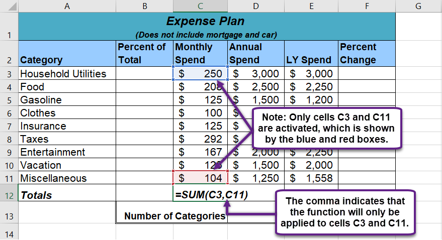
When you intend to use a statistical function on a range of cells in a worksheet, make sure there are two cell locations separated by a colon and not a comma. If you enter two cell locations separated by a comma, the function will produce an output, but it will be applied to only two cell locations instead of a range of cells. For example, the SUM function shown in Figure 2.8 will add only the values in cells C3 and C11, not the range C3:C11.
The COUNT Function
Data file: Continue with CH2 Personal Budget.
The next function that we will add to the Budget Detail worksheet is the COUNT function. The COUNT function is used to determine how many cells in a range contain a numeric entry. The COUNT function will not work for counting text or other non-numeric entries. For the Budget Detail worksheet, we will use the COUNT function to count the number of items that are planned in the Annual Spend column (Column D). The following explains how the COUNT function is added to the worksheet by using the function list:
- Click cell D13 in the Budget Detail worksheet.
- Type an equal sign =.
- Type the letter C.
- Click the down arrow on the scroll bar of the function list (see Figure 2.9) and find the word COUNT.
- Double click the word COUNT from the function list.
- Highlight the range D3:D11.
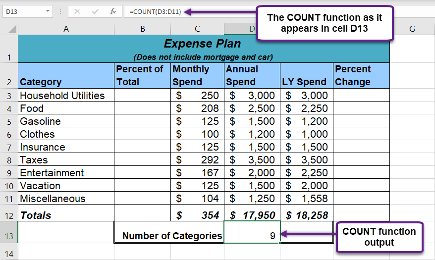
- You can type a closing parenthesis ) and then press the ENTER key, or simply press the ENTER key and Excel will close the function for you. The function produces an output of 9 since there are 9 items planned on the worksheet.
Figure 2.9 shows the function list box that appears after completing steps 2 and 3 for the COUNT function. The function list provides an alternative method for adding a function to a worksheet.
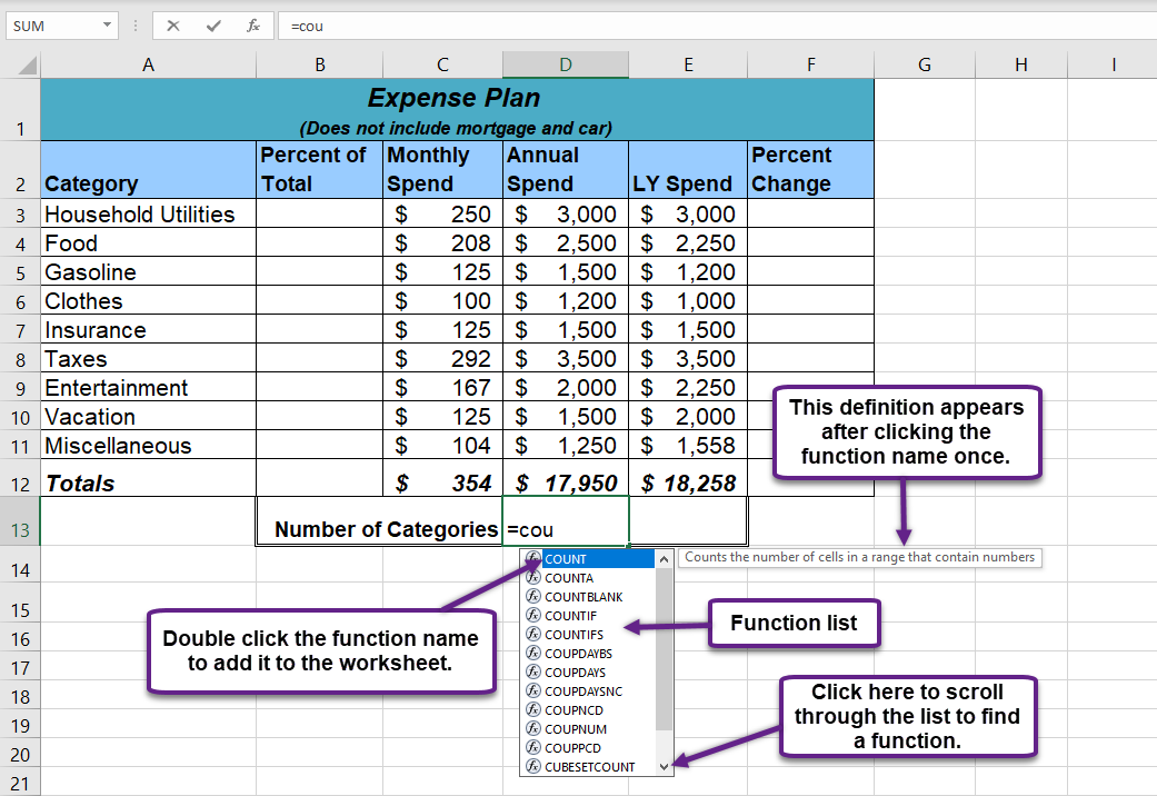
Figure 2.10 shows the output of the COUNT function after pressing the ENTER key. The function counts the number of cells in the range D3:D11 that contain a numeric value. The result of 9 indicates that there are 9 categories planned for this budget.
The COUNTA Function
The next function that we will use is the COUNTA function. The COUNT function counts how many cells in a range contain a numeric entry, whereas the COUNTA function is used to determine how many cells in a range contain numbers and text.
will not work for counting text or other non-numeric entries. For the Budget Detail worksheet, we will use the COUNT function to count the number of items that are planned in the Annual Spend column (Column D). The following explains how the COUNT function is added to the worksheet by using the function list:
- Click cell D13 in the Budget Detail worksheet.
- Delete the existing COUNT function.
- Type an equal sign =.
- Type the letter C.
- Click the down arrow on the scroll bar of the function list (see Figure 2.9) and find the word COUNTA.
- Double click the word COUNTA from the function list.
- Highlight the range A3:A11.
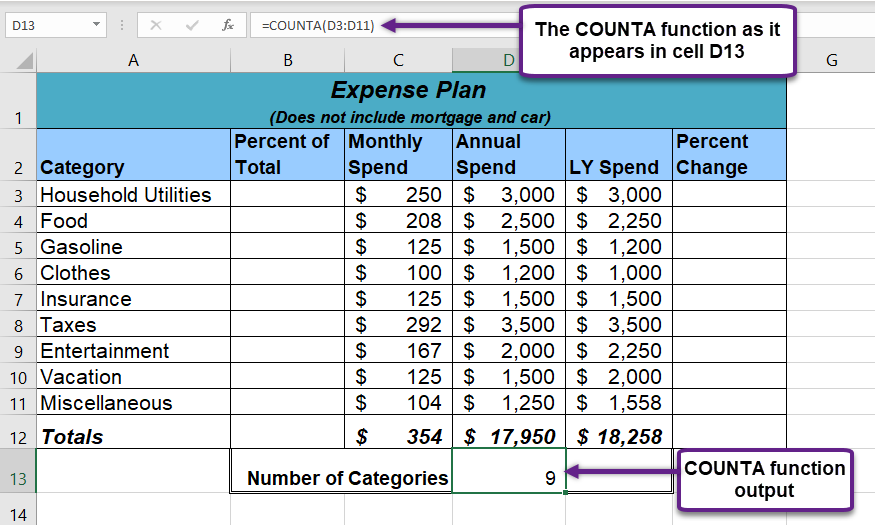
- You can type a closing parenthesis ) and then press the ENTER key, or simply press the ENTER key and Excel will close the function for you. The function produces an output of 9 since there are 9 items planned on the worksheet.
Figure 2.11 shows the function list box that appears after completing steps 2 and 3 for the COUNTA function. The function list provides an alternative method for adding a function to a worksheet.
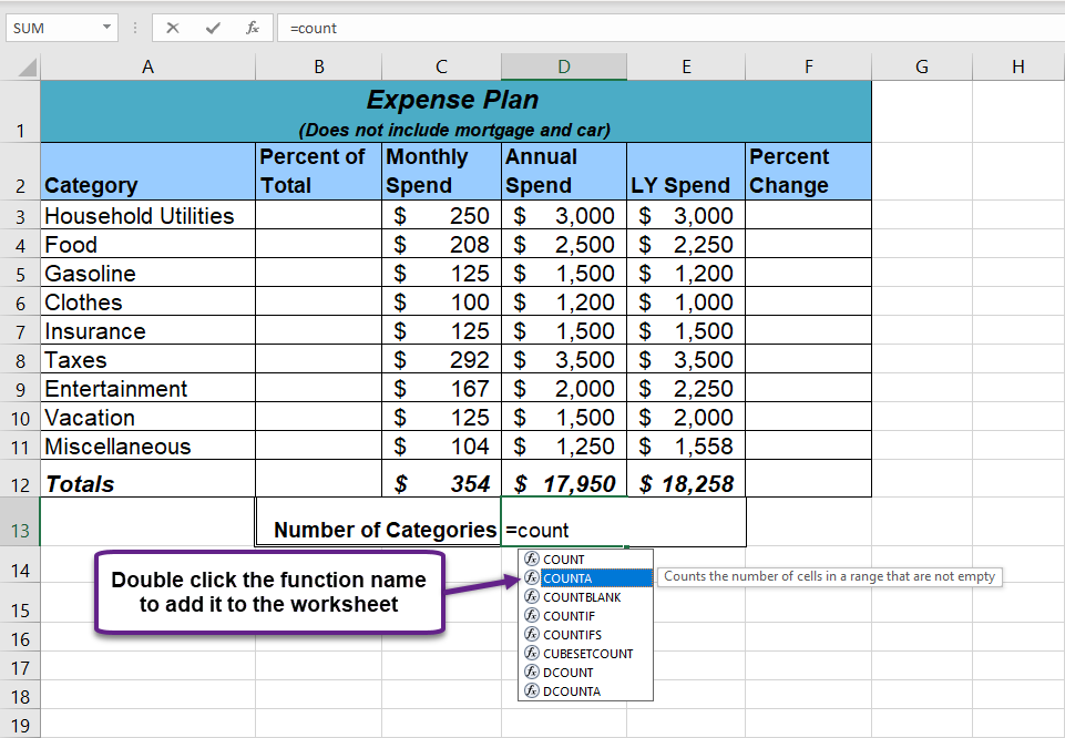
Figure 2.12 shows the output of the COUNTA function after pressing the ENTER key. The function counts the number of cells in the range D3:D11 that contain a either a numeric or text value (non-blank cells). The result of 9 indicates that there are 9 categories planned for this budget.
Skill Refresher
Statistical Functions:
- Type an equal sign =.
- Type the function name followed by an open parenthesis ( or double click the function name from the function list.
- Highlight a range on a worksheet or click individual cell locations followed by commas.
- Type a closing parenthesis) and press the ENTER key or press the ENTER key to close the function.
Copy and Paste Formulas (Pasting without Formats)
As shown in Figure 2.13, the COUNTA function are summarizing the data in the Annual Spend column. You will also notice that there is space to copy and paste these functions under the LY Spend column. This allows us to compare what we spent last year and what we are planning to spend this year.
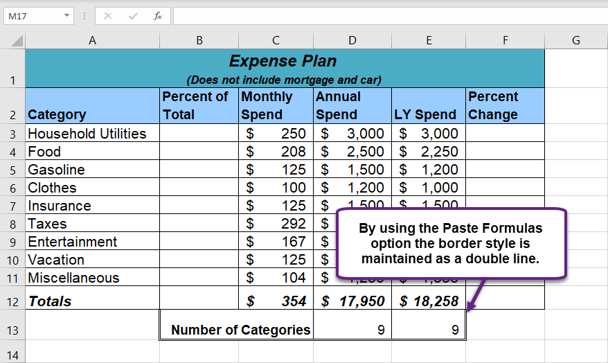
Normally, we would simply copy and paste these functions into the range E13:E16. However, you may have noticed the double-line style border that was used around the perimeter of the range B13:E16. If we used the regular Paste command, the double line on the right side of the range E13:E16 would be replaced with a single line. Therefore, we are going to use one of the Paste Special commands to paste only the functions without any of the formatting treatments. This is accomplished through the following steps:
- Highlight Cell D13 in the Budget Detail worksheet.
- Click the Copy button in the Home tab of the Ribbon.
- Click cell E13.
- Click the down arrow below the Paste button in the Home tab of the Ribbon.
- Click the Formulas option from the drop-down list of buttons (see Figure 2.13).
Figure 2.13 shows the list of buttons that appear when you click the down arrow below the Paste button in the Home tab of the Ribbon. One thing to note about these options is that you can preview them before you make a selection by dragging the mouse pointer over the options. As shown in the figure, when the mouse pointer is placed over the Formulas button, you can see how the functions will appear before making a selection.
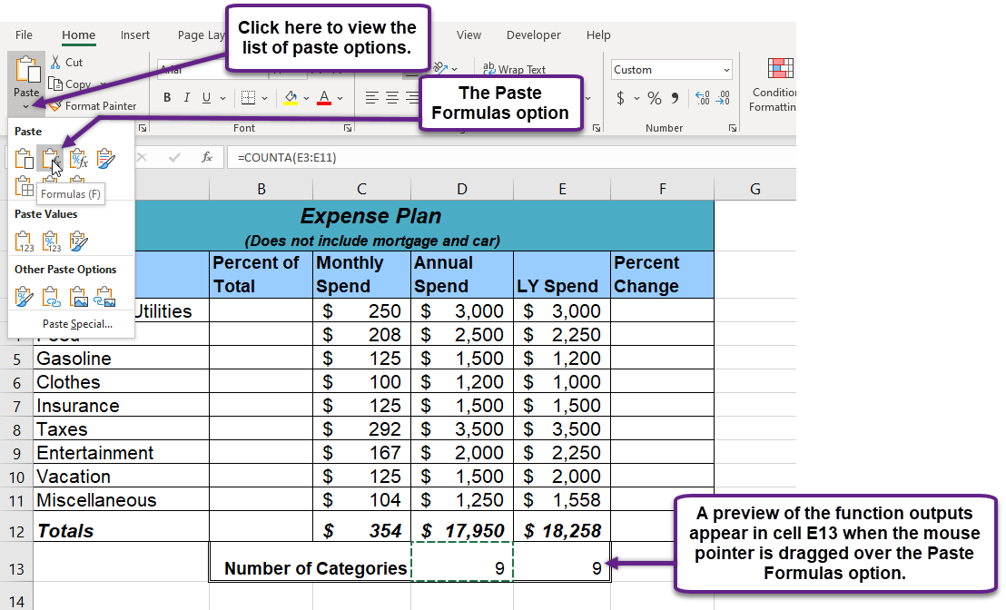
Figure 2.14 Notice that the double-line border does not change when this option is previewed. That is why this selection is made instead of the regular Paste option.
Skill Refresher
Paste Formulas:
- Click a cell location containing a formula or function.
- Click the Copy button in the Home tab of the Ribbon.
- Click the cell location or cell range where the formula or function will be pasted.
- Click the down arrow below the Paste button in the Home tab of the Ribbon.
- Click the Formulas button under the Paste group of buttons.
Error Messages
Sometimes Excel notices that you have made errors in your calculations before you do. In those cases Excel alerts you with some slightly mysterious error messages. A list of common error messages can be found in Table 2.5 below.
Table 2.4 – Common Error Messages |
|
Message |
What Went Wrong |
|
#DIV/0! |
You tried to divide a number by a zero (0) or an empty |
|
#NAME |
You used a cell range name in the formula, but the name isn’t |
|
#N/A |
The formula refers to an empty cell, so no data is available |
|
#NULL |
The formula refers to a cell range that Excel can’t understand. |
|
#NUM |
An argument you use in your formula is invalid. |
|
#REF |
The cell or range of cells that the formula refers to aren’t |
|
#VALUE |
The formula includes a function that was used incorrectly, |
Key Takeaways
- Statistical functions are used when a mathematical process is required for a range of cells, such as summing the values in several cell locations. For these computations, functions are preferable to formulas because adding many cell locations one at a time to a formula can be very time-consuming.
- Statistical functions can be created using cell ranges or selected cell locations separated by commas. Make sure you use a cell range (two cell locations separated by a colon) when applying a statistical function to a contiguous range of cells.
- The #DIV/0 error appears if you create a formula that attempts to divide a constant or the value in a cell reference by zero.
- The Paste Formulas option is used when you need to paste formulas without any formatting treatments into cell locations that have already been formatted.
