Chapter 5
Section 5.2 – Formulas with 3-D References
Learning Objectives
- Entering formulas that reference another sheet.
- Using the SUM function to add up multiple sheets.
- Grouping and ungrouping worksheets.
- Creating a summary worksheet using 3-D references.
The Summary sheet in many multiple sheet workbooks is utilized to present totaled information from the other sheets in the file. This is done to give a quick synopsis of all the other sheets in one convenient location. For this reason, the Summary sheet is usually the first sheet in multiple sheet files. Summary sheets “pull” data from the other sheets using three-dimensional (3-D) cell references. To distinguish between A3 in the Summary sheet, A3 in the January sheet, A3 in the February sheet, etc.; a 3-D cell reference includes the sheet name along with the cell reference. The syntax to reference a cell in a different sheet is =SheetName!CellRange. So, the cell reference for A15 in the March sheet would be =March!A15.
Continue using FILE: CH 5.1
Let us start working on our summary sheet by trying out some 3-D formulas:
- Click on the Expenses Summary sheet tab at the bottom of the screen.
- Click on C5 and enter the formula =January!C5. Press Enter.
This will get the amount $700 from cell C5 in the January sheet. - Delete the formula in C5 in the Expenses Summary sheet.
- This time click on C5 and type =. Then click on the January sheet, and then click on C5.
- Press Enter. This will put the same formula, =January!C5, in cell C5 in the Expenses Summary sheet and will return the value $700.
- In cell C6 in the Expenses Summary sheet, try entering a formula for the Power amount in the April sheet. You should get $135 as the Power amount.
- Delete the formulas in cells C5 and C6 in the Expenses Summary sheet.
For the Annual Amounts in C5:C13 in the Expenses Summary sheet, we do not need the amount from a single month’s sheets; instead, we need the sum of all the entries in all the monthly sheets. So, we need to sum three-dimensionally through all twelve-month sheets. Here is a helpful hint on the steps you need to follow to add through multiple sheets:
Skill Refresher
To SUM across sheets:
- Click on the cell where you want the 3-D SUM to appear.
- Type =SUM(
- Click on the leftmost sheet in the group of sheets you want to sum.
- Hold the SHIFT key down and click on the rightmost sheet in the group of sheets you want to sum.
- Click on the cell in the sheet you are in that you want to sum.
- Press ENTER.
Grouping and Ungrouping Sheets
The monthly budget sheets include a place in each of these sheets to calculate three pieces of Summary data: Income, Expenses, and Balance; but there are not any formulas in these cells. There is also a place for the % of Income Spent, but we need a formula in I6:I7 to calculate this. If we entered these formulas individually in each of the 12-month sheets, it would take a long time! Because this task would be very repetitive, it would also be likely that we would make some mistakes along the way entering the same formulas repeatedly. By grouping all the month sheets together, we can enter each of the formulas once and have them appear in all the sheets.
- Click on the January sheet to make it active.
- Hold the SHIFT key down and click on the December sheet.
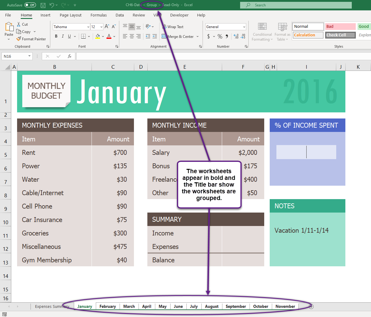
Now all 12 sheets should be selected. You can tell this in two ways: the sheet tabs that have been selected are now bold at the bottom of your screen. Notice in the Title bar at the top of the screen the word [Group] added to the end of the title. You can see both in Figure 5.4.
This is a very good thing when we want to make changes to all the sheets at once, but we need to be sure to ungroup them when we are done making these changes. Let’s go ahead and add the formulas to all twelve of the sheets at once:
- Click in F11 in the January grouped sheet.
- Enter the formula =SUM(F5:F8).
- In F12, enter the formula =SUM(C5:C13).
- In F13, subtract Expenses from Income. In the January sheet, your balance should be $690. HINT: if your answer is negative, you subtracted Income from Expenses.
- Click on I6. (I6 and I7 are formatted and merged – this is fine.)
- Enter a formula that divides Expenses (F12) by Income (F11). Your answer will show as a percentage since this cell has already been formatted to do this. HINT: If your percentage is greater than 100%, you have your numbers reversed.
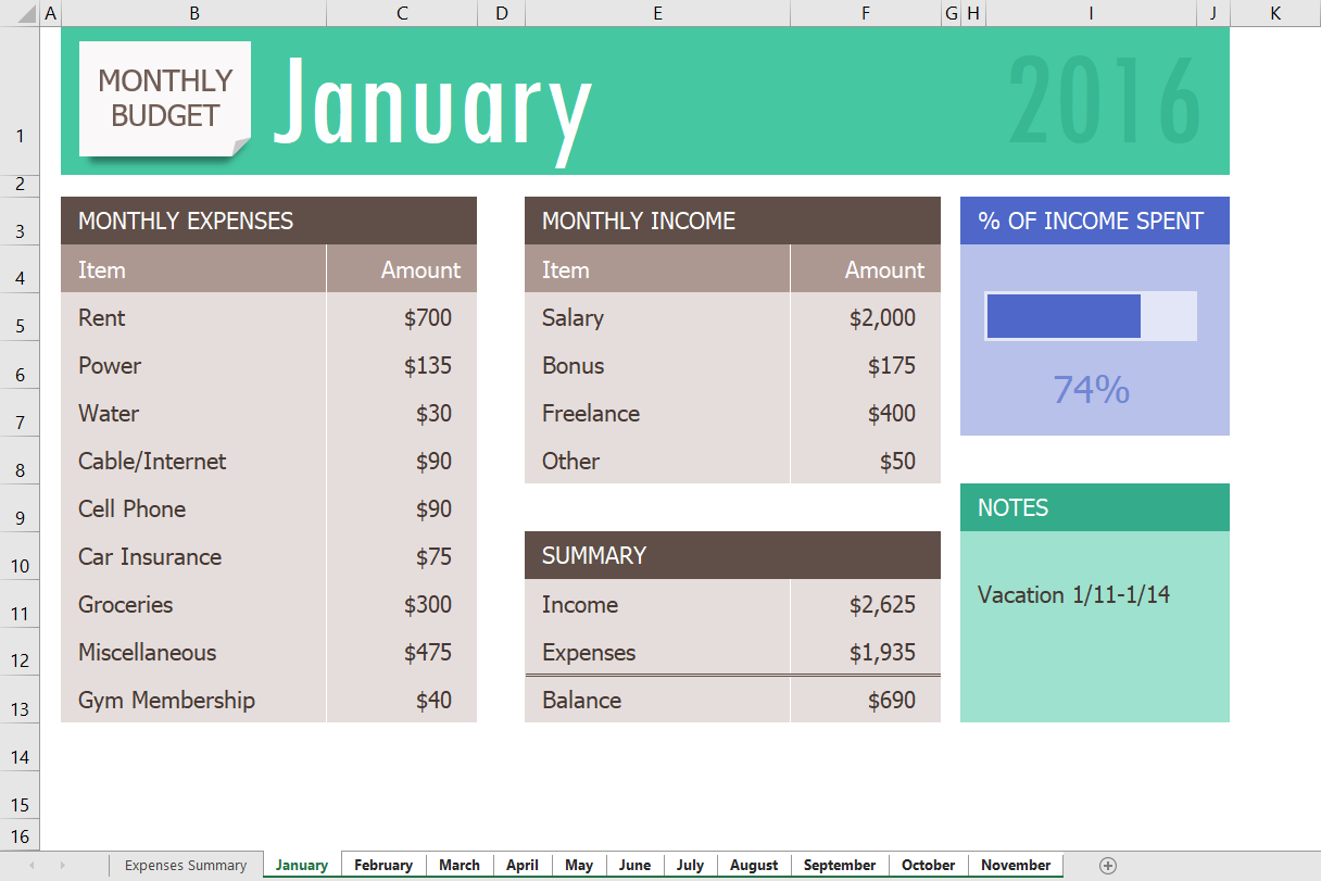
Notice that a data bar was set up in I5 to visually show the income spent. Do you remember how to do this from earlier in our textbook? Your January sheet should now look like Figure 5.5.
- Now that we are done making changes to all the monthly sheets at once, we need to ungroup them. Right-click on one of the grouped sheets and choose Ungroup Sheets.
Notice the sheets tabs are no longer bold and the word [Group] is no longer in the title bar.
- Click on several of the month sheets to see that all the formulas have been added.
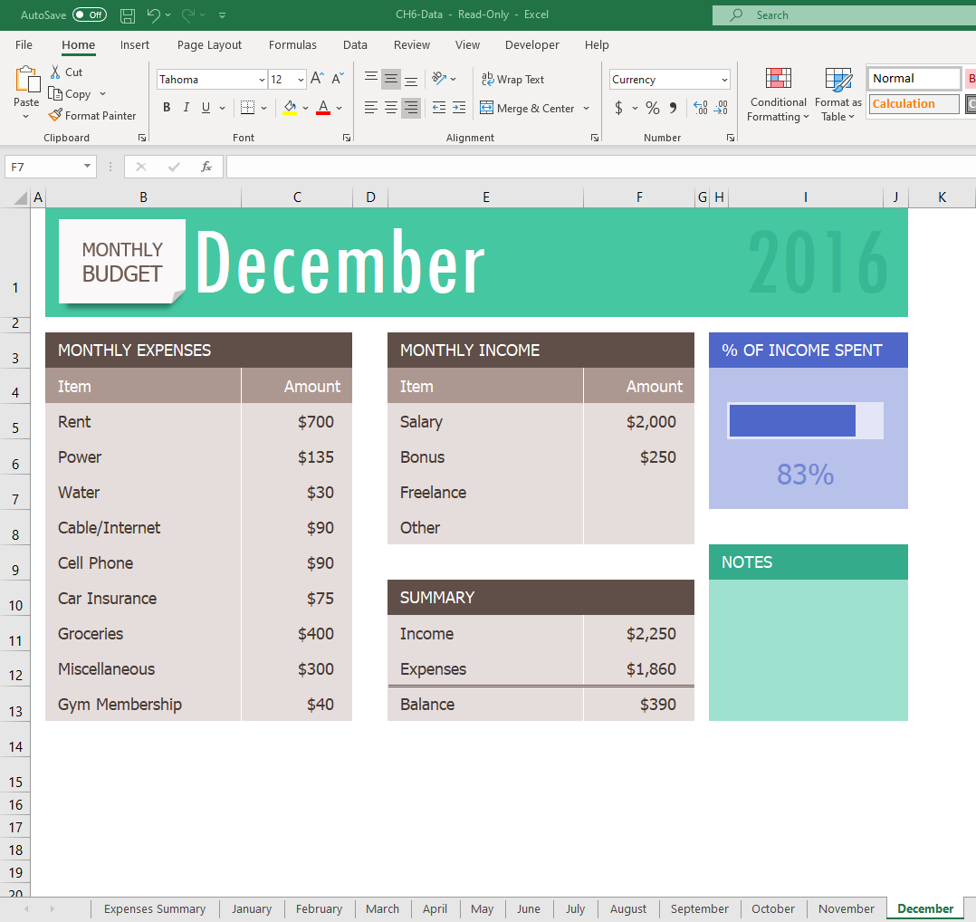
- Click on the December sheet. Your sheet should now look like Figure 5.6.
- Look at the Notes in the September sheet. It says that the rent was raised in September, so we need to cancel our Gym Membership and show $0 for the Gym amount in October, November, and December.
- Group the October, November, and December sheets. If you do this successfully, these three sheet names should be bold and the word [Group] will appear in the Title bar.
- Click on C13 and change the amount to $0. Press Enter.
- Ungroup the sheets. The balances should be: October $605, November $530, and December $430.
Skill Refresher
To Group Sheets:
- Click on the leftmost sheet you want to group; then hold the SHIFT key down and click on the rightmost sheet you want to group.
To Ungroup Sheets:
- Right-click on one of the grouped sheets and choose Ungroup Sheets.
Linking Worksheets (Creating a Summary Worksheet)
So far, we have used cell references in formulas and functions, which allow Excel to produce new outputs when the values in the cell references are changed. Cell references can also be used to display values or the outputs of formulas and functions in cell locations on other worksheets.
This is how data will be displayed on the Expense Summary worksheet in the workbook. Outputs from the formulas and functions that were entered into the January – December worksheets will be displayed on the Expense Summary worksheet using cell references. The following steps explain how this is accomplished:
- Click cell C5 in the Expense Summary worksheet.
- Type an equal sign and enter the SUM function =SUM.
- Group the January to December worksheets (select January then hold down shift and click December)
- Click in cell C5 and press the Enter key to finish the function.
You will notice that the sum of all the rents from January to December were calculated using this 3D cell reference. Your sum should be $8,400.
- Complete the remainder of the SUM functions on the Expense Summary worksheet.
Figure 5.7 shows how the cell reference appears in the Expense Summary worksheet. Notice that the cell reference C5 is preceded by the January:December! worksheet names followed by an exclamation point. This indicates that the value displayed in the cell C5 is referencing a cell locations in the January to December worksheets.
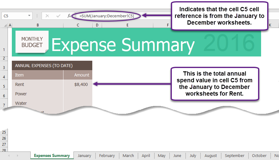
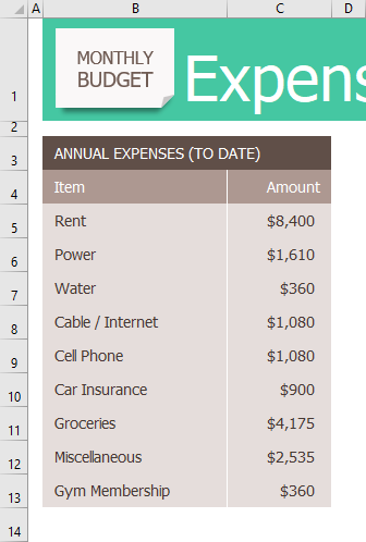
Figure 5.8 shows the results of creating formulas for the remaining expense categories in the Expense Summary worksheet.
We can now add other formulas and functions to the Expense Summary worksheet that can calculate the total yearly expenses. The following steps explain how this is accomplished:
- Click cell C14 in the Expense Summary worksheet.
- Type an equal sign =.
- Type the function name SUM followed by an open parenthesis (.
- Highlight the range C5:C13.
- Type a closing parenthesis ) and press the ENTER key on your keyboard or simply press the ENTER key to close the function. The total for all annual expenses now appears on the worksheet.
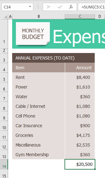
Figure 5.9 shows the results of the formula added to the Expense Summary worksheet. The output for the formula in cell C14 shows that the total yearly expenses were $20,500.
We can now add a few formulas that calculate the percentage each category of expense is of the total. These formulas require the use of absolute references. The following steps explain how to add these formulas:
- Click cell E5 in the Expense Summary worksheet.
- Type an equal sign =.
- Click cell C5.
- Type a forward slash / for division and then click C14.
- Press the F4 key on your keyboard. This adds an absolute reference to cell C14.
- Format the results as a percentage with 1 decimal place.
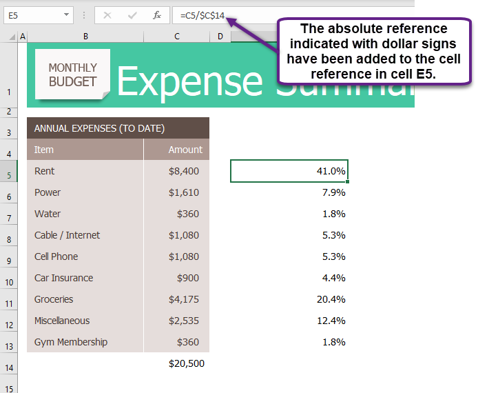
- Press the ENTER key. The result of the formula shows that Rent accounts for 41% of total yearly expenses.
- Complete the remaining expense category percent calculations.
Figure 5.10 shows the output of the formulas calculating the percentage of yearly expenses. The absolute reference shown for cell E5 prevents the cell from changing when the formula is copied from cell E6 to E13.
Key Takeaways
- Grouping sheets allows you to change a group of identically formatted sheets at the same time.
- 3-D references in formulas allow you to use data from one or more sheets on another sheet.
