Chapter 4
Section 4.1 – Creating Complex Formulas (Controlling the Order of Operations)
Learning Objectives
- Work with complex formulas by controlling the order of mathematical operations.
- Use the Smart Lookup tool to acquire additional information about percentage calculations.
- Review the use of Absolute cell reference in a division formula.
Download and open FILE: CH 4.1
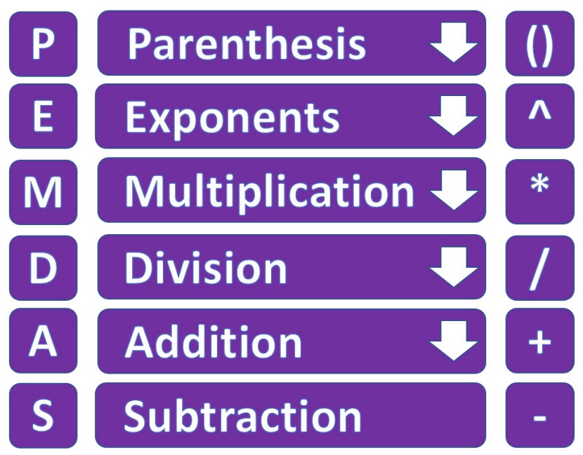
The next formula to be added to the Personal Budget workbook is the percent change over last year. This formula determines the difference between the values in the LY (Last Year) Spend column and shows the difference in terms of a percentage. This requires that the order of mathematical operations be controlled to get an accurate result. Table 4.1 shows the standard order of operations for a typical formula. To change the order of operations shown in the table, we use parentheses to process certain mathematical calculations first. This formula is added to the worksheet as follows:
Table 4.1 – Standard Order of Mathematical Operations |
|
Symbol |
Order |
|
( ) |
Override Standard Order: Any mathematical computations placed in parentheses are performed first and override the standard order of operations. If there are layers of parentheses used in a formula, Excel computes the innermost parentheses first and the outermost parentheses last. |
|
^ |
First: Excel executes any exponential computations first. |
|
* or / |
Second: Excel performs any multiplication or division computations second. When there are multiple instances of these computations in a formula, they are executed in order from left to right. |
|
+ or − |
Third: Excel performs any addition or subtraction computations third. When there are multiple instances of these computations in a formula, they are executed in order from left to right. |
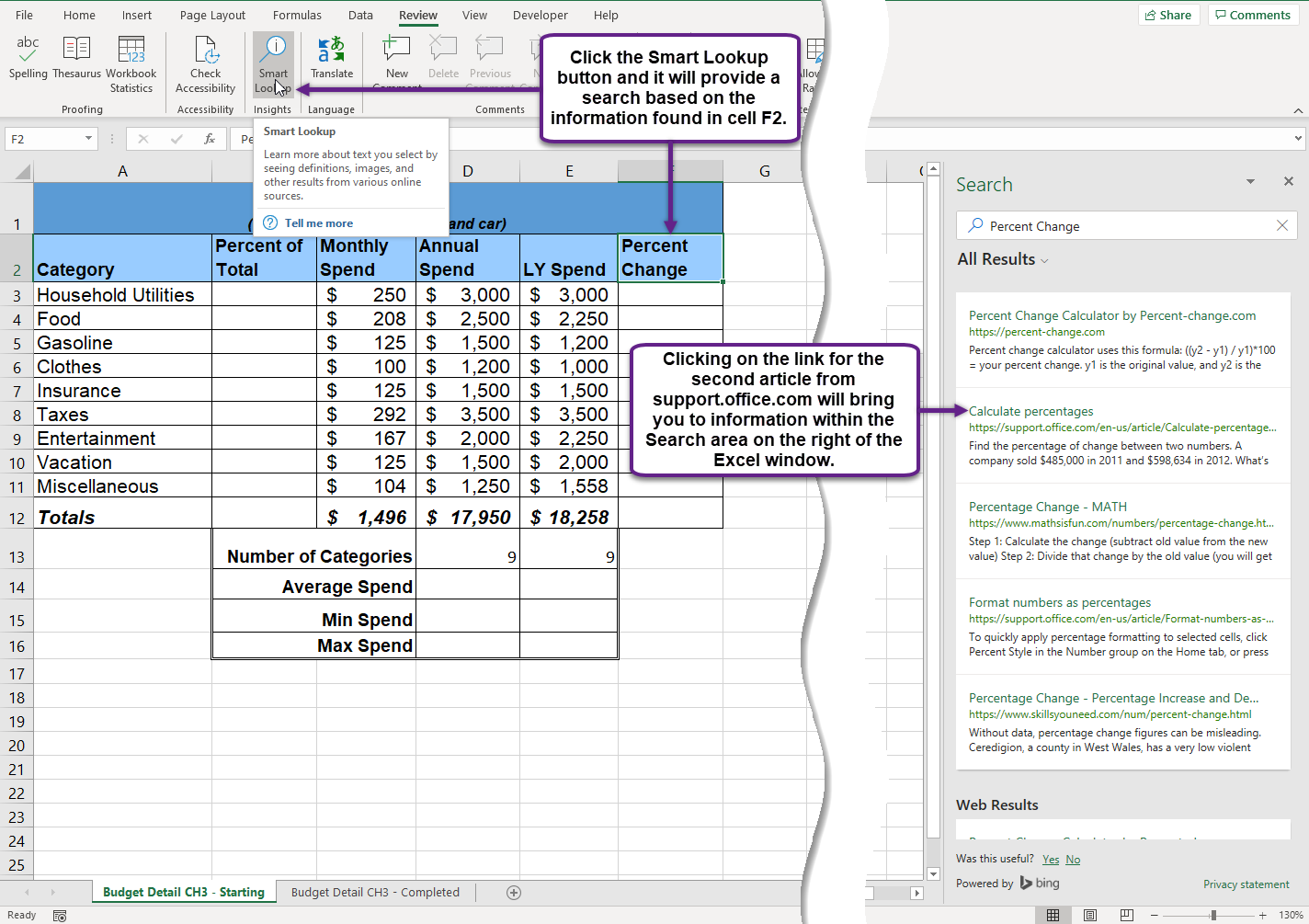
Using Smart Lookup
Column F requires a Percentage calculation. Before we launch in to creating a calculation for this, it might be handy to know precisely what it is we are looking for. If you are connected to the internet, and are using Excel 2016 or newer, you can use the Smart Lookup tool to get some more information.
- Select cell F2.
- Find the Smart Lookup tool on the Review tab (see Figure 4.1).
- Press the Smart Lookup tool to find more about Percentage calculations.
If this is the first time you have used the Smart Lookup tool, you may need to respond to a statement about your privacy. Press the Got it button.
I think the second article from Microsoft does a pretty good job explaining the calculation, don’t you?
Now that we know what is needed for the Percentage calculation, we can have Excel do the calculation for us. We need to divide the LY Spend for each category by the Annual Spend minus the LY Spend.
- Click cell F3 in the Budget Detail worksheet.
- Type an equal sign =.
- Type an open parenthesis (.
- Click cell D3. This will add a cell reference to cell D3 to the formula. When building formulas, you can click cell locations instead of typing them.
- Type a minus sign −.
- Click cell E3 to add this cell reference to the formula.
- Type a closing parenthesis ).
- Type the slash / symbol for division.
- Click cell E3. This completes the formula that will calculate the percent change of last year’s actual spent dollars vs. this year’s budgeted spend dollars (see Figure 4.2).
- Press the ENTER key.
- Click cell F3 to activate it.
- Place the mouse pointer over the Auto Fill Handle.
- When the mouse pointer turns from a white block plus sign to a black plus sign, click and drag down to cell F11. This pastes the formula into the range F4:F11.
Figure 4.2 shows the formula that was added to the Budget Detail worksheet to calculate the percent change in spending. The parentheses were added to this formula to control the order of operations. Any mathematical computations placed in parentheses are executed first before the standard order of mathematical operations (see Table 4.2). In this case, if parentheses were not used, Excel would produce an erroneous result for this worksheet.
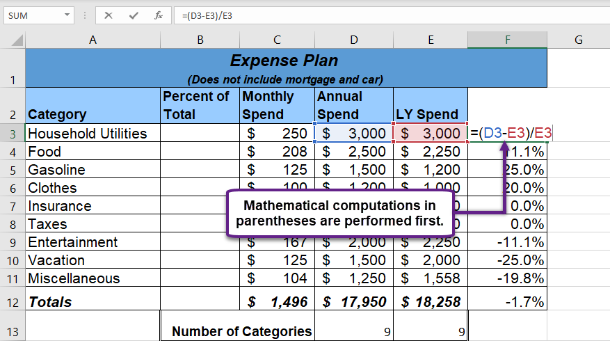
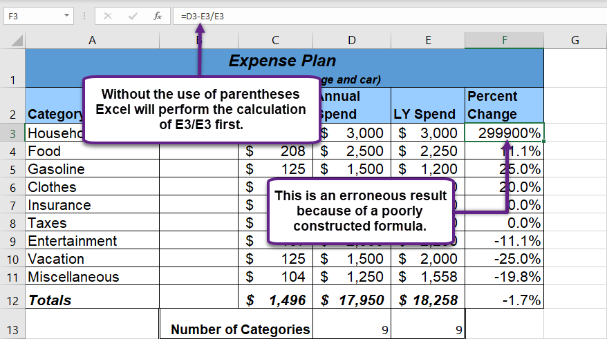
Figure 4.3 shows the result of the percent change formula if the parentheses are removed. The formula produces a result of a 299900% increase. Since there is no change between the LY spend and the budget Annual Spend, the result should be 0%. However, without the parentheses, Excel is following the standard order of operations. This means the value in cell E3 will be divided by E3 first (3,000/3,000), which is 1. Then, the value of 1 will be subtracted from the value in cell D3 (3,000−1), which is 2,999. Since cell F3 is formatted as a percentage, Excel expresses the output as an increase of 299900%.
Integrity Check
Does the Output of Your Formula Make Sense?
It is important to note that the accuracy of the output produced by a formula depends on how it is constructed. Therefore, always check the result of your formula to see whether it makes sense with data in your worksheet. As shown in Figure 4.3, a poorly constructed formula can give you an inaccurate result. In other words, you can see that there is no change between the Annual Spend and LY Spend for Household Utilities. Therefore, the result of the formula should be 0%. However, since the parentheses were removed in this case, the formula is clearly producing an erroneous result.
Skill Refresher
Formulas:
- Type an equal sign =.
- Click or type a cell location. If using constants, type a number.
- Type a mathematical operator.
- Click or type a cell location. If using constants, type a number.
- Use parentheses where necessary to control the order of operations.
- Press the ENTER key.
Absolute References (Calculating Percent of Totals)
Data file: Continue with CH2 Personal Budget.
Since totals were added to row 12 of the Budget Detail worksheet, a percent of total calculation can be added to Column B beginning in cell B3. The percent of total calculation shows the percentage for each value in the Annual Spend column with respect to the total in cell D12. However, after the formula is created, it will be necessary to turn off Excel’s relative referencing feature before copying and pasting the formula to the rest of the cell locations in the column. Turning off Excel’s relative referencing feature is accomplished through an absolute reference. The following steps explain how this is done:
- Click cell B3 in the Budget Detail worksheet.
- Type an equal sign =.
- Click cell D3.
- Type a forward slash /.
- Click cell D12.
- Press the ENTER key. You will see that Household Utilities represents 14.23% of the Annual Spend budget (see Figure 4.4).
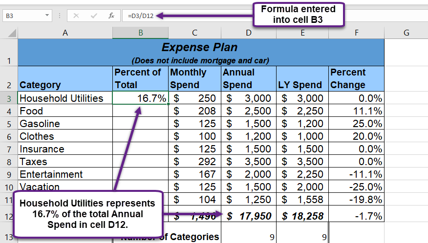
Figure 4.4 shows the completed formula that is calculating the percentage that Household Utilities Annual Spend represents to the total Annual Spend for the budget (see cell B3). Normally, we would copy this formula and paste it into the range B4:B11. However, because of relative referencing, both cell references will increase by one row as the formula is pasted into the cells below B3. This is fine for the first cell reference in the formula (D3) but not for the second cell reference (D12).
Figure 4.5 illustrates what happens if we paste the formula into the range B4:B12 in its current state. Notice that Excel produces the #DIV/0 error code. This means that Excel is trying to divide a number by zero, which is impossible. Looking at the formula in cell B4, you see that the first cell reference was changed from D3 to D4. This is fine because we now want to divide the Annual Spend for Insurance by the total Annual Spend in cell D12. However, Excel has also changed the D12 cell reference to D13. Because cell location D13 is blank, the formula produces the #DIV/0 error code.
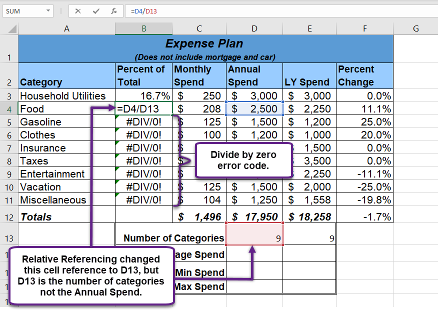
To eliminate the divide-by-zero error shown in Figure 4.5 we must add an absolute reference to cell D12 in the formula. An absolute reference prevents relative referencing from changing a cell reference in a formula. This is also referred to as locking a cell. The following explains how this is accomplished:
- Double click cell B3.
- Place the mouse pointer in front of D12 and click. The blinking cursor should be in front of the D in the cell reference D12.
- Press the F4 key. You will see a dollar sign ($) added in front of the column letter D and the row number 12. You can also type the dollar signs in front of the column letter and row number.
- Press the ENTER key.
- Click cell B3.
- Click the Copy button in the Home tab of the Ribbon.
- Highlight the range B4:B11.
- Click the Paste button in the Home tab of the Ribbon.
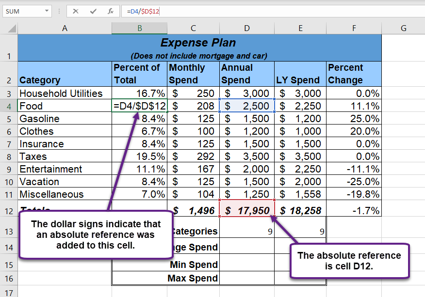
Figure 4.6 shows the percent of total formula with an absolute reference added to D12. Notice that in cell B4, the cell reference remains D12 instead of changing to D13 as shown in Figure 4.5. Also, you will see that the percentages are being calculated in the rest of the cells in the column, and the divide-by-zero error is now eliminated.
Skill Refresher
Absolute References:
- Click in front of the column letter of a cell reference in a formula or function that you do not want altered when the formula or function is pasted into a new cell location.
- Press the F4 key or type a dollar sign $ in front of the column letter and row number of the cell reference.
