Section 2.4 – Preparing to Print

Download and open File: CH 2.3

In this section, we will review some of the formatting techniques covered in Chapter 1, as well as learn some new techniques. We will also preview a two-page worksheet and set page setup options to present the data in a professional manner. A new data file will be used in this section.

Formatting Worksheet Data

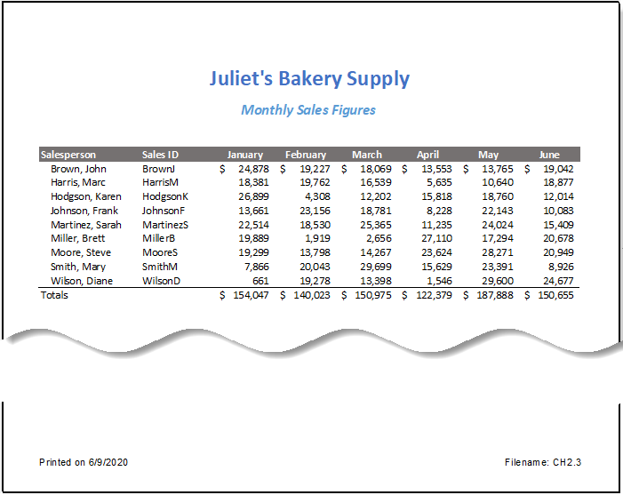
You have been given sales data that needs to be formatted in a professional manner. This worksheet will be printed and presented to investors, so it needs to be prepared for printing as well. Figure 2.23 shows how the finished worksheet will appear in Print Preview.

1. Open the Data file named CH2.3 and use the File/Save As command to save it with the new name CH2 Sales Data.
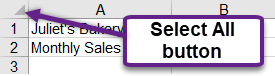
2. To change the font of the entire worksheet, click the Select All button in the top left corner of the worksheet grid (see Figure 2.24).

3. Change the font to Calibri, Size 12.
4. Using the skills learned in Chapter 1, make the following formatting changes:
   1. A1:H1 – Merge and Center; format text as bold and apply a font color and size of your choice, and change the Row height to 50
   2. A2:H2 – Merge and Center; format text as bold and italic, apply a font color of your choice
   3. A5:H5 – Apply a dark fill color; format text as white and bold
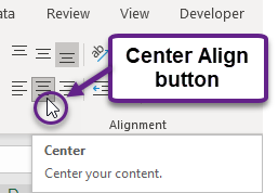
   4. C5:H5 – Center align (see Figure 2.25)

5. A15:H15 – Apply Top Border to the cells; format text as bold
6. C6:H6 and C15:H15 – Apply Accounting Number format with 0 decimal places
7. C7:H14 – Apply Comma style with 0 decimal places
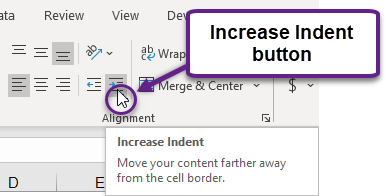
8. Highlight A6:A14 (salespeople’s names) and click the Increase Indent button in the Alignment group on the Home ribbon (see Figure 2.26). This will indent the text from the cell border.

Fine-tuning Formatting

Now that you have fixed the inconsistencies in the formatting, you decide to apply some formatting techniques to make the worksheet look even better. You are going to start by vertically aligning the names of the states within the cells.

1. Select cell A1
2. Click the Home tab on the ribbon.
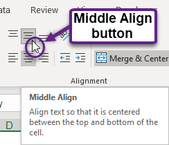
3. In the Alignment group, click the Middle Align button (see Figure 2.27). Notice that Juliet’s Bakery Supply is now centered between the top and bottom borders of the cell.

Using Page Setup Options

Once the worksheet is professionally formatted, you need to look in Print Preview to see how the pages will print.

1. With the CH2 Sales Data file still open, go to Backstage View by clicking the File tab on the ribbon. Select Print from the menu. Notice that the worksheet is currently printing on two pages, with the page breaking between the April and May columns. To fix this problem, you will first change the left and right margins while still in Print Preview
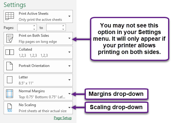
2. Click the Margins drop-down arrow in the Settings section (see Figure 2.28)
3. Select Custom Margins… at the bottom of the list.
4. Type in 0.5 for the Left Margin and 0.5 for the Right Margin.
5. Click OK. Changing the margins brought the May column onto the same page, but the June column is still on a separate page. Next you will use Page Scaling to fix this while still in Print Preview.
6. Click the Scaling drop-down arrow in the Settings section (Figure 2.28).
7. Select Fit All Columns on One Page.
8. Exit Backstage View.

Creating a Footer using Page Setup

Now that the entire worksheet is printing on one page, you need to add a footer with information about the date the file was printed along with the filename. In Chapter 1 you learned how to create headers and footers using the Insert ribbon. You can also create headers and footers using the Custom Header/Footer dialog box.

1. Click the Page Layout tab on the ribbon.
2. Click the dialog box launcher in the Page Setup group. A window similar to Figure 2.29 should appear.

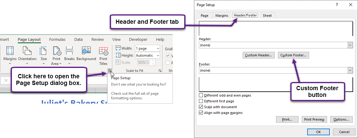
3. Click the Header/Footer tab in the Page Setup dialog box.
4. Click the Custom Footer button. The Footer dialog box should appear (see Figure 2.30).
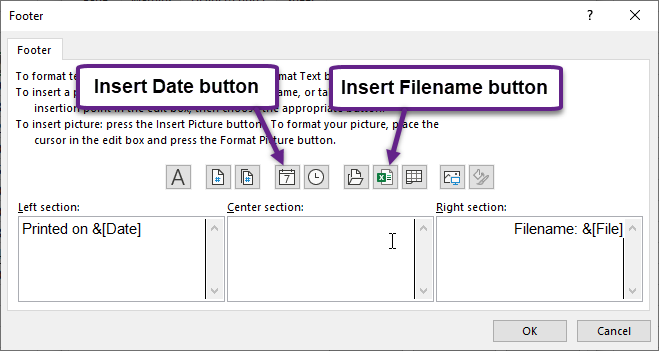
5. Click in the Left section: box and type Printed on.
6. Making sure to leave a space after the word on, click the Insert Date button.
7. Click in the Right section: box and type Filename:
8. Making sure to leave a space after the colon, click the Insert File Name button.
9. The Footer dialog box should look like Figure 2.30.
10. Click the OK button. Click OK again to close the Page Setup dialog box.
11. Go to Print Preview to see that the current date and file name are displayed in the footer.
12. Exit Backstage View. Save the CH2 Sales Data file.
13. Compare your work with the self-check answer key (found in the Course Files link) and then submit the CH2 Sales Data workbook as directed by your instructor.