Download and open FILE: CH 4.2

This section reviews the fundamental skills for setting up and maintaining an Excel table. The objective used for this chapter is the construction of tables in a multi-sheet file to keep track of two cities’ national weather data for the month of January. Organizing, maintaining, and reporting data are essentials skills for employees in most industries.

Figure 4.7 shows the completed workbook that will be demonstrated in this chapter. Notice that this workbook contains three worksheets. The first worksheet lists average weather for January in Portland, Maine. The second sheet lists average weather data for January in a very different climate – Portland, Oregon. The third sheet adds a weekly column to the Portland, Oregon data so that it can be subtotaled by week.

Creating a Table

When data is presented in long lists or columns, it helps if the table is set up well. Here are some rules of data-entry etiquette to follow when creating a table from scratch:

• Whenever you can, organize your information using adjacent (neighboring) columns and rows.
• Start the table in the upper-left corner of the worksheet and work your way down the sheet.
• Do not skip columns and rows just to “space out” the information. (To place white space between information in adjacent columns and rows, you can widen columns, heighten rows, and change the alignment.)
• Reserve a single column at the left edge of the table for the table’s row headings or identifying information.
• Reserve a single row at the top of the table for the table’s column headings.
• If your table requires a title, put the title in the row(s) above the column headings.

Following these rules will help ensure that the sorts, filters, totals, and subtotals you apply to your table with give you the desired results.

With these rules in mind, we will begin working on the Portland ME worksheet in the National Weather workbook. Notice that the data is in adjacent columns and rows. The upper-left corner of the table is in A5 and the titles are above the column headings in Row 5. Since the set-up of our data looks good, we are ready to turn our data range into an Excel table:

1. Open data file CH4.2 and save a file to your computer as CH4 National Weather.
2. Click on A5 in the Portland ME sheet.
3. Click the Table button in the Insert tab of the Ribbon.
   Figure 4.8 will appear on your screen.

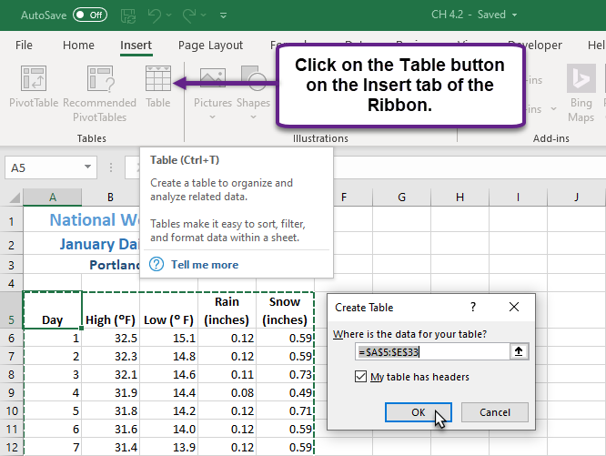
1. Make sure “My table has headers” is checked. Click OK.
2. Click in A5 again.
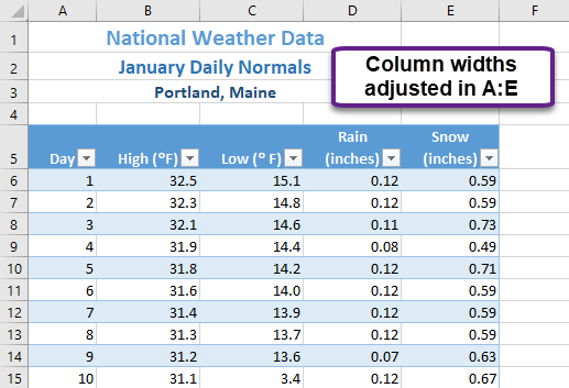
3. Adjust your columns widths so that you can see the complete headings in row 5 with the filter arrows showing. The filter arrows are the down-arrow buttons that will appear in row 5 when you create your table. We will learn how to use these to sort and filter later in this chapter.

After this, your spreadsheet will look like Figure 4.9.

Notice that a new ribbon tab, Table Tools Design, appears when you click inside your table. This ribbon tab allows you to edit, style, and add functionality to your table.

Let’s try a different way to create a table by following these steps:

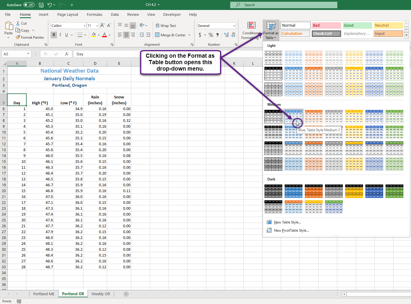
1. Click on the Portland OR sheet and click in cell A5.
2. Click the Format as Table button on the Home tab of the Ribbon.
3. Select Blue, Table Style Medium 2 option (see Figure 9.5).
4. Make sure “My table has headers” is checked. Click OK.
5. Click in A5 again.
6. Adjust your columns widths so that you can see the complete headings in row 5 with the filter arrows showing.

Formatting Tables

There are many ways to format an Excel table. There are preset colored Table Styles with Light, Medium, and Dark colors. There are also a variety of Table Style Options listed in Table 4.2.

Table 4.2 – Table Style Options
Table Style	Description
Header Row	Top row of the table that includes column headings
Total Row	Row added to the bottom that applies column summary calculations
First Column	Formatting added to the left-most column in the table
Last Column	Formatting added to the right-most column in the table
Banded Rows	Alternating rows of color added to make it easier to see rows of data
Banded Columns	Alternating columns of color added to make it easier to see columns of data
Filter Button	Button that appear at the top of each column that lists options for sorting and filtering

We will add some formatting to both of our Portland weather tables in the following steps:

1. Click on the Portland ME sheet in your file.
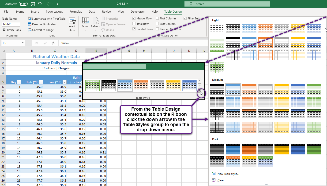
2. In the Table Tools Design tab, in the Table Styles group, click the More button.
3. A gallery of table styles will appear as in Figure 4.10.

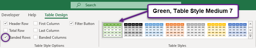
4. In the Table Styles gallery, in the Medium Section, click Green,Table Style Medium 7.
5. In the Table Style Options group in the Ribbon, click Banded Rows.
6. The alternating colored rows will disappear. The data in the table is now more difficult to read.
7. Try out some of the other options in the Table Style Options group. Once you’re finished, check just Header Row, Banded Rows, and Filter Button as in Figure 4.11 below.

Freeze Rows and Columns

When you freeze panes, Microsoft Excel keeps specific rows or columns visible in your table when you scroll through it on your screen. For example, if the first row in your spreadsheet contains labels, you might freeze that row to make sure that the column labels remain visible as you scroll down in your spreadsheet. When we scroll through our weather data, it would be nice to keep our column headings visible on the screen.

To freeze your headings:

1. Click on the Portland ME sheet in your file.
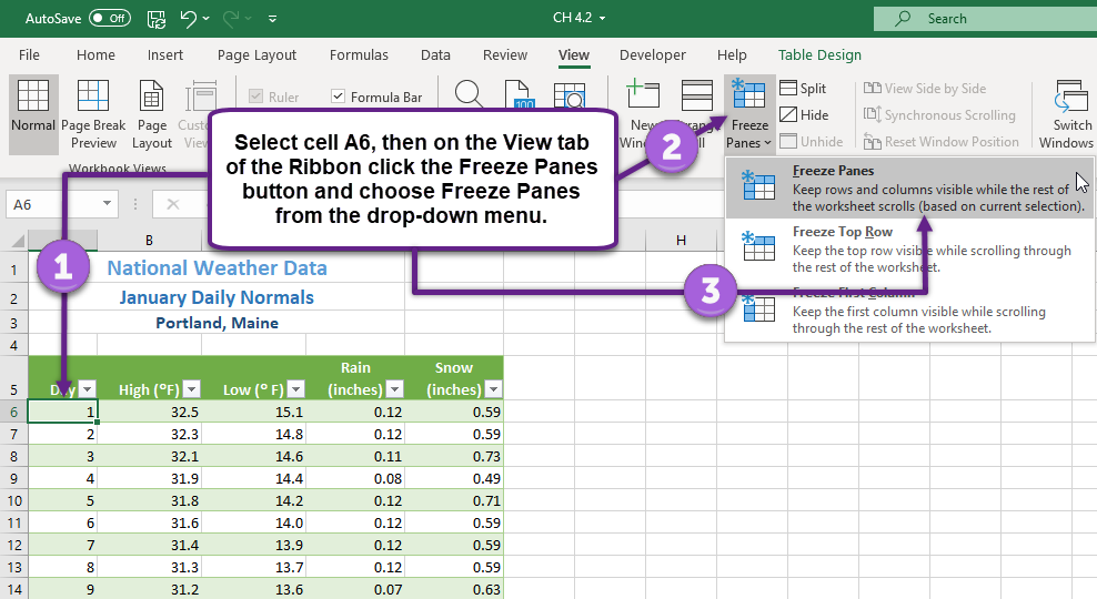
2. Click in A6, the left-most cell below the headings row.
3. Click the View tab in the ribbon.
4. Select Freeze Panes and then Freeze Panes again.
5. Scroll up and down the sheet and notice that the headings are always displayed at the top of the table.

To unfreeze your headings:

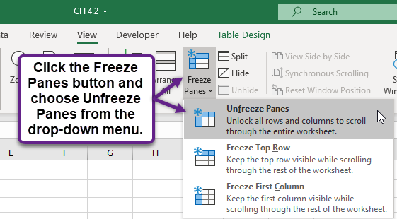
1. Click on the View tab in the ribbon.
2. Select Unfreeze Panes.

Simple Sort

Content in a table can be sorted alphabetically, numerically, and in many other ways. Sorting helps organize data by one or more columns in your table. Table 4.3 describes the different sort orders available for each column of data.

Table 4.3 – Sort Options
Sort Order	Text	Numbers	Dates
Ascending	Alphabetical (A-Z)	Smallest to Largest Lowest to Highest	Chronological (oldest to newest)
Descending	Reverse Alphabetical (Z-A)	Largest to Smallest Highest to Lowest	Reverse Chronological (newest to oldest)

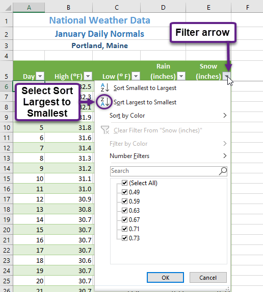
Let’s say we want to know what the snowiest day was in January in Portland, Maine; so we want to sort the Snow column in Descending order so that the snowiest day ends up at the top of the table.

1. Click on the filter Click arrow to the right of the header Snow (inches) in the Portland ME worksheet.
2. Click on the choice Click ZA↓ Sort Largest to Smallest. See Figure 4.13 below.

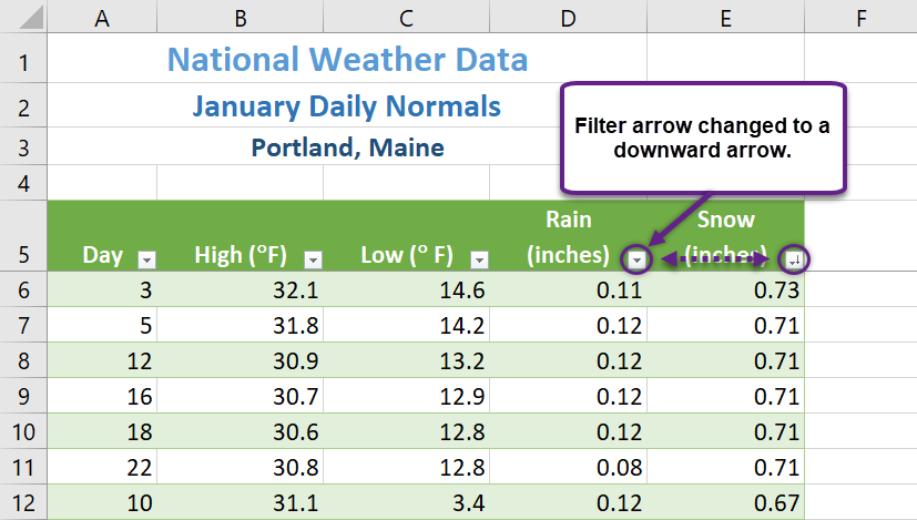
If you did this correctly, you will see that the snowiest day at the top of the list in January 3rd (in row 6) with 0.73 inches of snow! Notice the filter arrow changes in the snow column to a downward pointing arrow to indicate you sorted that column in descending order (largest to smallest).

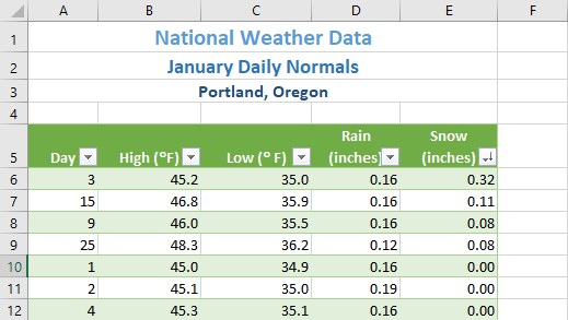
3. Now switch to the Portland Oregon sheet and repeat these sort steps to find the snowiest day in Oregon. Check your answers with Figure 4.15.

Filtering Data

When you first create an Excel table, filter arrows appear in all the column headings. We have seen that you can use those arrows to sort your data by a single column. You can also use these same arrows to filter or limit the data you see by narrowing the displayed data within a column. There are many ways to filter data within a column depending on whether the data in the column is text or numeric. Table 4.4 gives you some filter examples:

Table 4.4 – Filter Examples
Text Filters
Desired Results	Filter Column	Text Filter	Checkbox Selected
Data for the State of New Jersey (NJ)	State	Equals NJ	NJ
Data for Books that Have Gardening in Their Title	Title	Contains Gardening
Data for Weather on the Weekend	Day	Equals Saturday OR equals Sunday	Saturday and Sunday
Numeric Filters
Desired Results	Filter Column	Number Filter	Checkbox Selected
Data for Income Greater Than $1,000	Income	Greater than 1,000
Data for Amount Paid Equal to Zero	Amount Paid	Equals 0.00	0.00
Data for Mortgage and Auto Loans	Loan Type	Equals Mortgage OR equals Auto	Mortgage and Auto

Notice there are sometimes more than one way to filter data (i.e. – with a filter choice or a checked box). There are also single criteria filters, as well as, multi-criteria filters. We will explore all of these next.

To start filtering, let’s look at just the first week of data in the Weekly OR sheet:

1. Click on the Weekly OR sheet and click on a cell in the table.
2. Format the data range to a table, using Green, Table Style Medium 7,
3. Click the filter arrow to the right of the Week heading.
4. Click the Select All checkbox to deselect all of the checkbox choices.
5. Click on 1 to select Week 1.
6. Click OK.

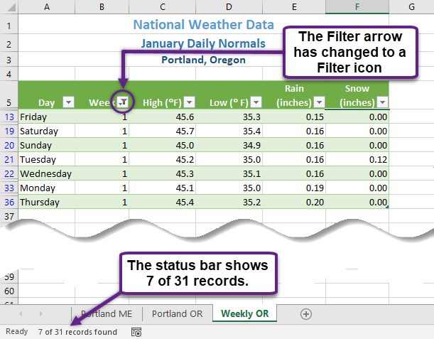
Your table should look like Figure 4.16. You should see only 7 rows of Week 1 data in your table. Notice in your Status Bar at the bottom of your screen the message “7 of 31 records found”. Also notice that the filter arrow in the Week heading has changed to a funnel which indicates that this column is currently filtered.

To remove your filter:

1. Click the funnel next to the Week heading.
2. Select “Clear filter from Week”.

 Now let’s try a numeric filter. We want to find days in Portland ME when it’s warmer than 32 degrees in January:

1. Click in the Portland ME sheet, then click on a cell in the table.
2. Click on the filter arrow next to the High heading.
3. Click on Number filters, then select Greater than. The Custom AutoFilter dialog box will appear on your screen.
4. Enter 32 in the space to the right of “is Greater than”. Your Custom AutoFilter dialog box should now match Figure 4.17.

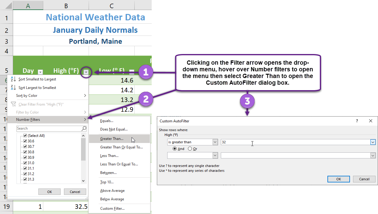
5. Click OK.

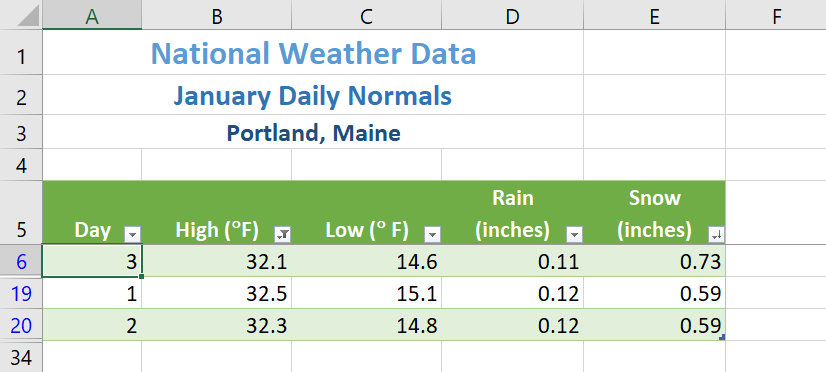
You should see that it was only above 32 degrees three days in January in Maine – the first three! Check your table against Figure 4.18.

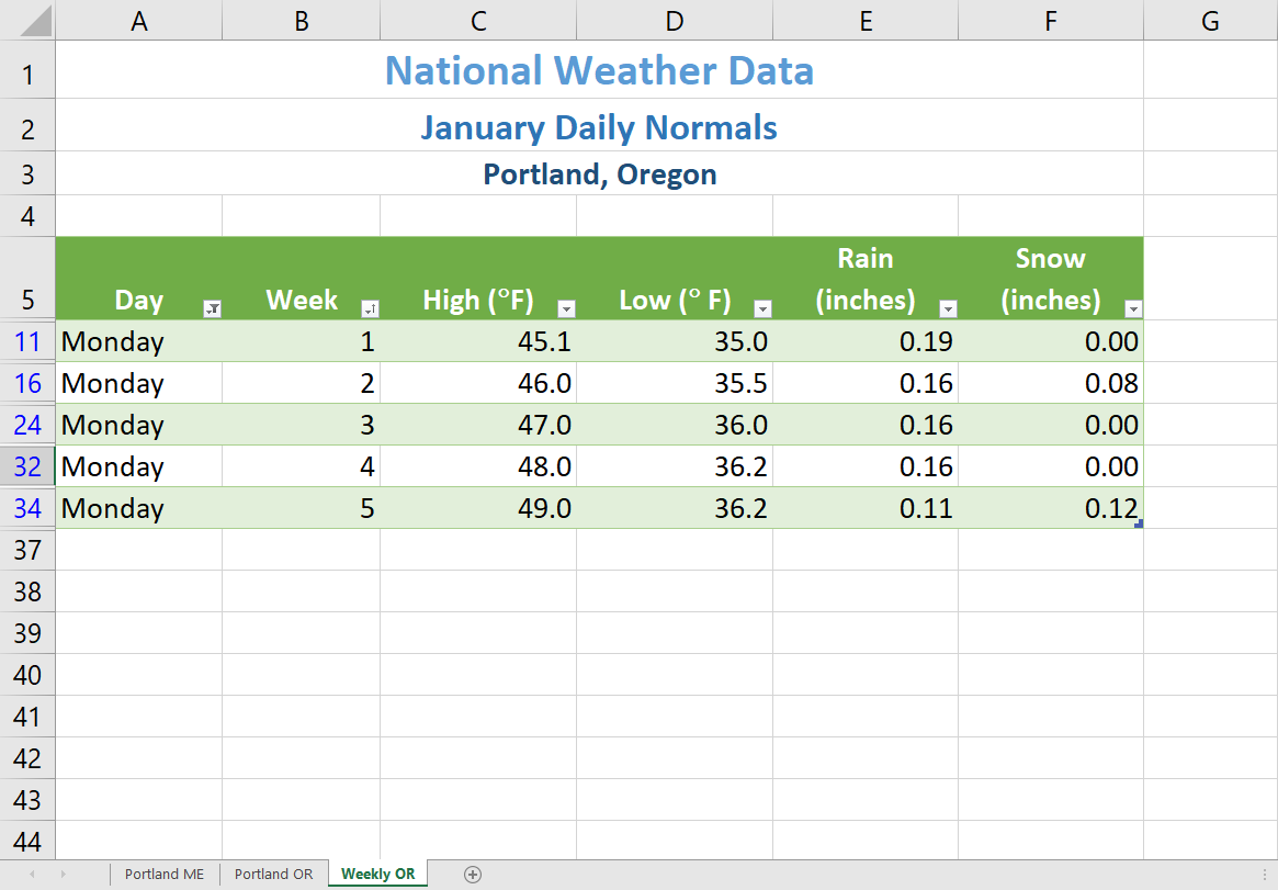
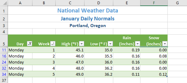
Let’s review sorting and filtering in the following steps:

1. Click on the Weekly OR sheet and clear the Week column filter.
2. Sort the table by Week (smallest to largest).
3. Filter the table to only show Mondays.
4. Compare your table results to Figure 4.19.